506  Active Crossover System Design

Figure 17.2: Gain structure for the preamplifier-crossover-power amplifier chain: (a) internal crossover level of 0 dBu gives an S/N ratio of 84.9 dB; (b) raising the internal level to +8 dBu gives an S/N ratio of 92.5 dB, an improvement of 7.6 dB.

at a still higher level, say 5 Vrms (we want to keep a little safety margin), with the signal more heavily attenuated at the output to reduce it to 0 dBu; the internal crossover signals would then be another 8 dB higher, and we should now get some 16 dB more signal-to-noise ratio than with the 0 dBu internal level.

If there are full-range level controls between the crossover outputs and the power amplifiers, to allow level trimming, then the operator may unwisely set them for a considerable degree of attenuation; they will probably then crank up the input into the crossover to compensate, so there is now a higher nominal level in the crossover to obtain the same final output level. This means that the headroom in the crossover is reduced, and the option of running it at a deliberately elevated internal level to improve the signal-noise ratio now looks less attractive. The question here is whether the noise performance should be compromised by increasing the headroom to allow for maladjustment.

Placing the Output Attenuator

Let’s stick for the moment with the situation that there are no full-range level controls on the power amplifiers, just an output level trim, as described earlier. We therefore have our passive attenuator at the crossover outputs. The signal has therefore been brought back down to something of the order of 1

Vrms before it passes along the interconnection between crossover and power amplifier. However—if the attenuator is placed at the destination end of the interconnect cable, as in Figure 17.3a, any hum and interference picked because of currents flowing through the cable ground will also be attenuated.

Ideally the output attenuator should be actually inside the power amplifier, as in Figure 17.3b, as this would also deal with any voltages caused by ground current flowing through the connector earth pins, but this requires a specialised amplifier design which would have a low input impedance and low overall gain. Its input parameters would have to be defined by a Domestic Electronic Crossover

Standard, and unless there was some sort of input switching, it would not be usable as an ordinary power amplifier.Abetter idea is to put the attenuator inside the connector that plugs into the power amp.

508  Active Crossover System Design

useful information, but it does not directly tell us what we want to know, which might typically be phrased as: “If I have a 3-way system with crossover frequencies at 500 Hz and 3 kHz, how much level can I expect in each of the three crossover bands?” Greiner and Eggars do however at the end of their paper summarise the spectral energy levels in each octave band, which is more helpful. See Table 17.1, which gives the levels in dB with respect to full CD level for eight different musical genres, and the average of them all. The frequencies are the centres of the octave bands.

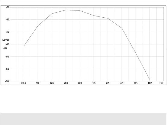
Figure 17.4 shows how the average levels are distributed across the audio band. The maximal levels are the region 100 Hz–2 kHz, with roll-offs of about 10 dB per octave at each end of the audio spectrum.

All we have to do is to decide which of the octave bands fit into our crossover bands and sum the levels in those bands to arrive at a composite figure for each crossover band.Apuzzling difficulty is to decide how to sum them—should they be treated as correlated (so two −6 dB levels sum to 0 dB) or uncorrelated (two −3 dB levels sum to 0 dB)?At first it seems unlikely that there would be much correlation between the octave bands, but on the other hand harmonics from a given musical instrument are likely to spread over several of them, giving some degree of correlation. I tried both, and for our purposes here the results are not very different.

Let’s assume that our LF crossover band includes the bottom four octave bands (31.5 to 250 Hz), the MID crossover band includes the middle three octave bands (500 Hz to 2 kHz), and the HF crossover band includes the top three octave bands (4 kHz to 16 kHz). Uncorrelated summing gives us

Table 17.2, where the actual levels in each crossover band are on the left and the relative levels of the

MID and HF bands compared with the LF band are in the two columns on the right.

Looking at the bottom line, the average of all the genres, we see that in general the MID crossover band will have similar levels in it to the LF crossover band. This is pretty much as expected, though it’s always good to have confirmation from hard facts. We also see that the average HF level is a heartening 11 dB below the other two crossover bands, so it looks as if we could run the HF channel at an increased level, say +10 dB, and get a corresponding improvement in signal-to-noise ratio.

Table 17.1: Spectral energy levels in octave bands for different genres (after Greiner and Eggars).

Active Crossover System Design  509

Figure 17.4: Average spectral levels in musical signals from CDs (after Greiner and Eggars).

Table 17.2: Uncorrelated sums of levels in the three crossover bands; HF band = top three octaves. The two columns on the right are levels relative to the 31.5–250 Hz LF band.

However . . . look a little deeper than the average. Table 17.2 shows that the HF level is significantly lower in all cases except for “Heavy Metal”, where the MID and HF levels are the same. This is so unlike all the other data that I am not convinced it is correct. It looks as though we could indeed run the HF channel a good 10 dB hotter if it were not for the existence of Heavy Metal—a sobering thought.

If we change our assumptions, moving the upper crossover frequency higher so that the MID crossover band now includes the middle four octave bands (500 Hz to 4 kHz) and the HF crossover