Добавил:

ivanov666 Опубликованный материал нарушает ваши авторские права? Сообщите нам.

Вуз:

Башкирский Государственный Аграрный Университет

Предмет:

[НЕСОРТИРОВАННОЕ]

Файл:

акустика / lin_h_bengisu_t_mourelatos_zp_lecture_notes_on_acoustics_and.pdf

Скачиваний:

154

Добавлен:

04.05.2023

Размер:

12.68 Mб

Скачать

☆

<<< < Предыдущая 53 54 55 56 57 58 59 60 61 62 63 6465 / 7865 66 67 68 69 70 71 72 73 74 75 76 77 > Следующая >>>

288

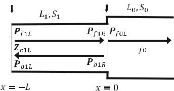
Power Transmission in Pipelines

P f 1R ¼ 2

1 þ Zc2L

Pc2L

ðFormula 4AÞ

Z f 1

Pb1R ¼ 2

1 Zc2L

Pc2L

ðFormula 4BÞ

Z f 1

Pb1R

Zc2L Z f 1

Formula 4C

P f 1R ¼

Zc2L

Z f 1

Pc2L

2Zc2L

ðFormula 4DÞ

P f 1R

Zc2L

Z f 1

where:

Pc2L ¼ P f 2L þ Pb2L

ðFormula 1DÞ

P f 2L þ Pb2L

Formula 3A

c2L ¼

f 2 P f 2L

Pb2L

Z f 2 ¼ ρoc

Note that when there is only an outward wave in Pipe 2 (Pb2L ¼ 0), Pc2L ¼ Pf2L and Zc2L ¼ Zf2.

11.5Transformation of Acoustic Impedance

Formula 5

Acoustic Impedance in the Reﬂected Pipe

The combined acoustic impedance Zc1L at the LHS of Pipe 1 can be calculated from Zc2L at the LHS of Pipe 2 as:

Z		=Z	Zc2L þ jZ f 1 tan ðkL1Þ	ð	Formula 5	Þ
	c1L		f 1 jZc2L tan ðkL1Þ þ Z f 1

where:

Z f 1 ¼ ρoc

Proof of Formula 5

Based on Formula 3A, the acoustic impedance Zc1L at the LHS of Pipe 1 is given as:

jkL1

ejkL1

Pb1R

e jkL1

Zc1L = Z f 1

P f 1Re

þ Pb1Re

=Z f 1

þ P f 1R

P f 1RejkL1

2Pb1Re jkL1

Pb1R

ejkL1 2

jkL1

P f 1R

11.5 Transformation of Acoustic Impedance				289
According to Formula 4C,	Pb1R	¼	Zc2L Z f 1	, the equation above can be
	P f 1R		Zc2LþZ f 1

rearranged as:

Zc2L

Z e

Z 2Z e

jkL1

Zc2L Z f 1

jkL1

Zc1L =Z f 1

þ f 1

=Z f 1

c2L þ

f 1

jkL1 þ

c2L

f 1

jkL1

Zc2L

Z f 1

Zc2L

þZ f 1 e

jkL1

Zc2L

Z f 1

2 Zc2L 2Z f 1

Divide both the numerator and denominator by ejkL1

þ e jkL1

as:

Zc2L

Z f 1

ejkL1

e jkL1

Zc1L =Z f 1

jkL1

=Z f 1

ðe 1

e 1

jkL1

ejkL1

e jkL1

jkL

jkL1

Zc2L

Z f 1

jkL

Zc2L

Þ þ

Z f 1

þ Z f 1

Zc2L ðejkL1 þe jkL1 Þ

because:

sin ðkL1Þ

ejkL1

e jkL1

jkL1

tan

kL1

Þ ¼

¼ ejkL1

¼ j

cos ðkL1Þ

þ2e jkL1

ejkL1

þ e jkL1

Therefore, the combined acoustic impedance Zc1L at the LHS of Pipe 1 can be

calculated from Zc2L at the LHS of Pipe 2 as:
Z = Z			Zc2L þ jZ f 1 tan ðkL1Þ					ð	Formula 5	Þ
	c1L	f 1 jZc2L tan		ð	kL1	Þ þ	Z f 1
	c1L	f 1 jZc2L tan			kL1		Z f 1
where:
			Z f 1 ¼			ρoc
			Z f 1 ¼			S1

This concludes the proof of the formula for combined acoustic impedance in the pipe.

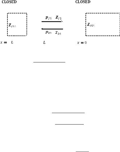
Two Special far End Boundary Conditions Case 1: Closed End Case Pf1R = Pb1R

The relationship above between the forward wave Pf1R and backward wave Pb1R can be obtained by Formula 4C for closed end (ZcoL ¼ 1) as:

P f 1R	¼	ZcoL þ Z f 1		ð	Formula 4C	Þ

Pb1R		ZcoL	Z f 1

Substitute ZcoL ¼ 1 into Formula 4C as:

290								11 Power Transmission in Pipelines
	P f 1R		ZcoL	Z f 1			Z f 1		ρoc
	P f 1R		ZcoL	Z f 1			Z f 1		1 þ S1
		¼		þ	¼	1	þ	¼		¼ 1
	Pb1R	¼	ZcoL	Z f 1	¼	1	Z f 1	¼	ρoc	¼ 1
						1			1 S1

! P f 1R = Pb1R

where ZcoL ¼ 1 due to the closed far end at x ¼ 0 (special case of Zc0Lfor the closed end boundary condition).

The same relationship between the forward wave and backward wave can be obtained by the conservation of mass for the closed end boundary condition as:

	P f 1R	U f 1R þ Ub1R ¼ 0				P f 1R	ðconservation of massÞ
		Pb1R		¼ 0				Pb1R	¼ 0	! P f 1R =Pb1R
!		þ			!		2	Z f 1
	Z f 1		Zb1			Z f 1

Case 2: Open End Case :Pf1R = 2 Pb1R

The relationship above between the forward wave Pf1R and backward wave Pb1R


can be obtained by Formula 4C for open end (ZcoL ¼ 0) as:
	PfR	ZcoL þ Z f 1			Formula 4C
PbR ¼				ð		Þ
		ZcoL	Z f 1

Substitute ZcoL ¼ 0 into Formula 4C as:

PfR	¼	ZcoL þ Z f 1		¼	0 þ Z f 1		¼	1

PbR		ZcoL	Z f 1		0	Z f 1

! P f 1R = 2Pb1R

where ZcoL ¼ 0 due to the far open end at x ¼ 0 (special case of Zc0Lfor the open end boundary condition).

The same relationship between the forward wave Pf1R and backward wave Pb1R can be obtained by balancing pressure for the open end boundary condition ( Pf0L ¼ Pb0L ¼ 0 at the outside of an open end pipe) as:

P f 1R þ Pb1R ¼ P f 0L þ Pb0L

ðstate of equilibriumÞ

!P f 1R þ Pb1R ¼ 0

!P f 1R = 2Pb1R

Four Combinations of the Complex Acoustic Impedances for the Special far End Conditions Stated Above and the Special Near end Conditions Below:

• General case of Zc2L:

Pc2L

Pf 2L þ Pb2L

general case

c2L Uc2L

Uf 2L

Ub2L

f 2 Pf 2L

Pb2L

11.5 Transformation of Acoustic Impedance

291

• Special case of Zc2Lfor closed end boundary condition (Uc2L ¼ 0):

Zc2L ¼	Pc2L	¼	Pc2L	¼ 1	ðclosed endÞ
	Uc2L		0

• Special case of Zc2L for open end boundary condition (Pc2L ¼ 0):

Zc2L ¼	Pc2L	0		¼ 0	ðopen endÞ
		¼
	Uc2L		Uc2L

Consider a single pipe with a ﬁnite length L. Assume the acoustic impedance at the near end is Zc1L and the acoustic impedance at the far end is Zc2L as shown in the ﬁgure above.

The four combinations of the complex acoustic impedances Zc1L and Zc2L of a single pipe for special end conditions are shown below:

	Near end: (x ¼ L )	Far end: (x ¼ 0)
Case 1	CLOSED: Zc1L = 1	CLOSED: Zc2L = 1
Case 2	OPEN: Zc1L = 0	OPEN: Zc2L = 0
Case 3	OPEN: Zc1L = 0	CLOSED: Zc2L = 1
Case 4	CLOSED: Zc1L = 1	OPEN: Zc2L = 0

	Pipe 1		Pipe 0

near end		far end
		far end

For case 1 and case 2, the detail calculations based on the combined acoustic impedance are given in Example 11.1 and 11.2. Case 3 and case 4 will be left as two exercises. Note that the results are identical to the solutions in Examples 7.1 and 7.2.

292	11 Power Transmission in Pipelines

Example 11.1: (Case 1: Closed-Closed)

For Case 1: a pipe with a CLOSED near end and a CLOSED far end

Near end		Pipe 1	Far end	Pipe 0
				Pipe 0
	= ∞			= ∞

The relationship between Zc1L of Pipe 1 and Zc0L of Pipe 0 is:
Z	=Z	Zc0L þ jZ f 1 tan ðkLÞ					ð	Formula 5	Þ
c1L		f 1 jZc0L tan	ð	kL	Þ þ	Z f 1	ð		Þ
			ð		Þ þ

The mode shapes are related to the wavenumber k that satisﬁes the given two boundary conditions:

Near end: CLOSED: Zc1L = 1 at x ¼ L Far end: CLOSED: Zc0L = 1 at x ¼ 0

Substituting Zc1L = 1 and Zc0L = 1 into the relationship between Zc1L of Pipe 1 and Zc0L of Pipe 0 yields:

Zc1L = Z f 1		Zc0L þ jZ f 1 tan ðkLÞ
		jZc0L tan ðkLÞ þ Z f 1

! 1	=Z f 1		Zc0L þ 0
			jZc0L tan ðkLÞ þ 0

Note that the two terms with Zf1are negligible because Zc0L is inﬁnite. Rearranging the above equation gives:

2jZ f 1

jZ f 1

cos ðkLÞ

tan

sin

! sin ðknLÞ = 0

and n ¼ 1, 2, 3, ∙ ∙ ∙

where kn ¼ n L ,

The resonant frequencies (ωn ¼ 2πfn ¼ ckn) are:

ckn

, where n

¼ 1, 2, 3, ∙ ∙ ∙

f n ¼

n L

2π

11.5 Transformation of Acoustic Impedance

293

And at these resonant frequencies ωn ¼ ckn, the mode shapes of the pressure with eigenfrequencies obtained above are:

p =P f 1Re jð kxÞ þ Pb1Re jðkxÞ

=P f 1Re jð kxÞ þ P f 1Re jðkxÞ

= P f 1R e jð kxÞ þ e jðkxÞ

=2P f 1R cos ðknxÞ

¼P cos nLπ x , where n ¼ 1, 2, 3, ∙ ∙ ∙

where the complex amplitude Pb1R is equal to the complex amplitude Pf1R as:

P f 1R ¼ Pb1R

The relationship above between the forward wave Pf1R and backward wave Pb1R can be obtained by Formula 4C for closed end (ZcoL ¼ 1) as shown in Example 11.2 as:

P f 1R	¼	ZcoL þ Z f 1		ð	Formula 4C	Þ

Pb1R		ZcoL	Z f 1

Substitute ZcoL ¼ 1 into Formula 4C as:

P f 1R		ZcoL	Z f 1			Z f 1		ρoc
P f 1R		ZcoL	Z f 1			Z f 1		1 þ S1
	¼		þ	¼	1	þ	¼		¼ 1
Pb1R	¼	ZcoL	Z f 1	¼	1	Z f 1	¼	ρoc	¼ 1
					1			1 S1

! P f 1R = Pb1R

Hence, the ﬁrst three modes of pressure in the pipe of the closed-closed ends are: Mode 1:

	πc	π	π		2π
ω1 ¼	L	; p1ðxÞ ¼ P cos L x ; k1	¼ L	¼		! λ1 ¼ 2L
					λ1

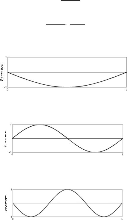
294	11 Power Transmission in Pipelines

Mode 2:

= −									=
	2πc	2π				2π		2π
ω2 ¼		; p2ðxÞ ¼ P cos		x ; k2	¼		¼		! λ2 ¼ L
ω2 ¼	L	; p2ðxÞ ¼ P cos	L	x ; k2	¼	L	¼	λ2	! λ2 ¼ L

Mode 3:

= −										=
	πc		3π			3π		2π		2
ω3 ¼	3	; p3ðxÞ ¼ P cos		x ; k3	¼		¼		! λ3 ¼		L
ω3 ¼	L	; p3ðxÞ ¼ P cos	L	x ; k3	¼	L	¼	λ3	! λ3 ¼	3	L

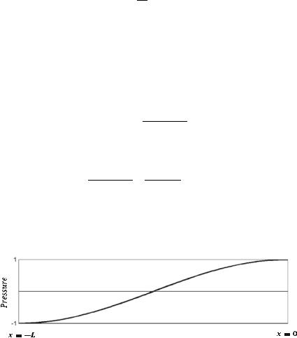
Example 11.2 (Case 2: Open-Open)

For Case 2: a pipe with an OPEN near end and an OPEN far end

Near end	Pipe 1	Far end	Pipe 0
			Pipe 0
= 0			= 0

11.5 Transformation of Acoustic Impedance

295

The relationship between Zc1L of Pipe 1 and Zc0L of Pipe 0 is:
Z	=Z	Zc0L þ jZ f 1 tan ðkLÞ					ð	Formula 5	Þ
c1L		f 1 jZc0L tan	ð	kL	Þ þ	Z f 1	ð		Þ
			ð		Þ þ

The mode shapes are related to the wavenumber k that satisﬁes the given two boundary conditions:

Near end: OPEN: Zc1L = 0 at x ¼ L Far end: OPEN: Zc0L = 0 at x ¼ 0

Substituting Zc1L = 0 and Zc0L = 0 into the relationship between Zc1L of Pipe 1 and Zc0L of Pipe 0 yields:

Zc1L = Z f 1			Zc0L þ jZ f 1 tan ðkLÞ
Zc1L = Z f 1			jZc0L tan ðkLÞ þ Z f 1
			jZc0L tan ðkLÞ þ Z f 1
!	0 = Z	f 1	0 þ jZ f 1 tan ðkLÞ
!		f 1	0	þ	Z f 1
				þ

! jZ f 1 tan ðkLÞ =0

The eigenfrequencies that satisfy the above equation are:

sin ðknLÞ =0 where kn ¼ n Lπ and n ¼ 1, 2, 3, ∙ ∙ ∙

The resonant frequencies (ωn ¼ 2πfn ¼ ckn) are:

f n ¼ ck2πn ¼ 2cπ n Lπ ¼ 2cnL , where n ¼ 1, 2, 3, ∙ ∙ ∙

And at these resonant frequencies ωn ¼ ckn, the mode shapes of the pressure with eigenfrequencies obtained above are:

p = P f 1Re jð kxÞ þ Pb1Re jðkxÞ

= P f 1Re jð kxÞ P f 1Re jðkxÞ

= P f 1R e jð kxÞ e jðkxÞ

= 2jP f 1R sin nLπ x , where n ¼ 1, 2, 3,

where the complex amplitude Pb1R is equal to the complex amplitude Pf1R as:

P f 1R ¼ 2Pb1R

The relationship above between the forward wave Pf1R and backward wave Pb1R can be obtained by Formula 4C for open end (ZcoL ¼ 0, based on Formula 4C) as:

296 11 Power Transmission in Pipelines

P f 1R	¼	ZcoL þ Z f 1		ð	Formula 4C	Þ

Pb1R		ZcoL	Z f 1

Substitute ZcoL ¼ 0 into Formula 4C as:

P f 1R	¼	ZcoL þ Z f 1		¼	0 þ Z f 1		¼	1

Pb1R		ZcoL	Z f 1		0	Z f 1

! P f 1R = 2Pb1R

Hence, the ﬁrst three modes of the pipe for the open-open ends are: Mode 1:

	πc	π	π		2π
ω1 ¼	L	; p1ðxÞ ¼ P sin L x ; k1	¼ L	¼		! λ1 ¼ 2L
					λ1

Mode 2:

ω2 ¼	2πc	; p2ðxÞ ¼ P sin	2π	x ; k2 ¼	2π	¼	2π		! λ2 ¼ L
	L		L		L			λ2

Mode 3:

11.6 Power Reﬂection and Transmission

297

ω3 ¼	3πc	; p3ðxÞ ¼ P sin	3π	x ; k3 ¼	3π	¼	2π	! λ3 ¼	2	L
	L		L		L		λ3		3

11.6Power Reﬂection and Transmission

11.6.1 Deﬁnition of Power of Acoustic Waves

The power of an acoustic wave is calculated from the pressure and velocity as the following:

(POWER) worktime ¼(PRESSURE) forcearea (VELOCITY) distanceime (AREA) [area]

Note that the work in the above equation is the force multiplied by the distance (work ¼ force distance):

Based on the above deﬁnition of power, the power of the acoustic wave is:

w ¼ Re ðPÞ Re ðVÞS ¼ Re ðPÞ Re ðUÞ

Re P Re Z			4		P P	Z		Z
	P		1			P		P
¼ ð Þ		¼		ð	þ Þ		þ

11.6.2Power Reﬂection and Transmission Coefﬁcients of One-to-One Pipes

Formulas 6A–6B

The power reﬂection and

transmission

coefﬁcients

in one-to-one

pipes are

deﬁned as:

Re ðPrÞ Re Zr

Formula 6A

¼ Re ðPiÞ Re

Re ðPoÞ Re Zo

Formula 6B

Re ðPiÞ Re

298	11 Power Transmission in Pipelines

, in general, can be a real or complex number

11.6.3Simpliﬁed Cases of Power Reﬂection and Transmission in One-to-One Pipes

Based on the deﬁnition of power transmission:

Tw	wo			Re ðPoÞ Re	Zo
					Po
			¼
	w	i	¼	Re ðPiÞ Re	Zi
	w				Pi

The following two simpliﬁed formulas can be derived for the relevant conditions: If Zi and Zo are real:

	½ Re ðPoÞ&2	Zi
Then, Tw ¼	½ Re ðPiÞ&2	Zo.

If Zi, Zo and Pi are real:

Then, Tw ¼ h Re Poi2 Zi .

Pi Zo

11.6.4Special Case of Power Reﬂection and Transmission: One-to-One Pipes

Formulas 7A–7E

Power of Traveling Plane Waves

Power reﬂection and transmission in one-to-one pipes can be formulated with real acoustic impedance Z and real magnitude P as:

2	1	ðFormula 7AÞ
wi ¼ Pi
	Zi

11.6 Power Reﬂection and Transmission

299

ðFormula 7BÞ

wr ¼ Pr

Rw ¼ wi

¼ Zo

ðFormula 7CÞ

¼ Pi

2 Zi

2Zo

2 Zi

Tw ¼

ðFormula 7DÞ

wi þ wr ¼ wo

ðFormula 7EÞ

where, for traveling plane waves, the following quantities are real numbers:

Zi, Zo, Pi, Po real

, , , real

Proof of Formulas 7A and 7B

For traveling plane waves (forward and backward) in pipes:

•The acoustic impedance Z is a real number.

•The complex amplitude of pressure P is also a real number.

Therefore, Formula 7A for the power of acoustic waves can be formulated with real acoustic impedance Z and real magnitude P as:

w ¼ Re ðPÞ Re P ¼ P2 1

Z Z

Because Zr ¼ Zi (Formula 1B), when the power is formulated with Zi, the power carried by the forward wave Pi and backward wave Pr are formulated as:

		2	1
wi ¼ Pi
wi ¼ Pi			Zi
2	1		2	1
wr ¼ Pr		¼ Pr
wr ¼ Pr	Zr	¼ Pr		Zi

300 11 Power Transmission in Pipelines

Proof of Formulas 7C and 7D

The power reﬂection and transmission coefﬁcients are deﬁned as:

Rw	wr			Re ðPrÞ Re	Zr
					Pr
			¼
	w	i	¼	Re ðPiÞ Re	Zi
	w				Pr
Tw	wo			Re ðPoÞ Re	Zo
					Po
			¼
	w	i	¼	Re ðPiÞ Re	Zi
	w				Pr

Because the following quantities for traveling plane waves in one-to-one pipes are real numbers:

Zi, Zr, Zo, Pi, Po real numbers

and:

Zr ¼ Zi

ðFormula 2BÞ

Therefore, the power reﬂection and transmission coefﬁcients can be simpliﬁed as:

Re ðPrÞ Re Zr

Pi2

Re ðPiÞ Re Zi

Re ðPoÞ Re Zo

2 Zi

Pi2

Re ðPiÞ Re Zi

Based on Formulas 4C–4D:

Pb1L

ZfoL Z f 1

P f 1R

¼ ZfoL

Z f 1

PfoL

2ZfoL

P f 1R

¼ ZfoL

Z f 1

ðFormula 4CÞ

ðFormula 4DÞ

The power reﬂection and transmission coefﬁcients can be formulated as:

Rw ¼ wi

¼ Zo

ðFormula 7CÞ

¼ Pi

2 Zi

2Zo

2 Zi

Tw ¼

ðFormula 7DÞ

11.6 Power Reﬂection and Transmission

301

Proof of Formula 7E

Based on the law of conservation of energy, the power that goes into a system has to equal the power that comes out of it:

(POWER IN) ¼ (POWER OUT)

Therefore, the summation of power on the left-hand side pipe equals the summation of power on the right-hand side pipe:

wi þ wr ¼ wo

ðFormula 7EÞ

Divide the equation above by wi to obtain the power ratio:

1 þ wr ¼ wo wi wi

!1 þ Rw ¼ Tw

!Rw þ Tw ¼ 1

Note that wi and wo does positive work but wr does negative work due to the negative impedance (180 phase difference between the pressure and the velocity).

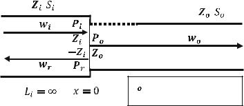
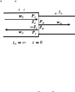
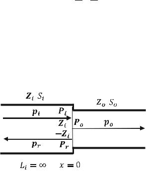
Example 11.3: Power Transmission Coefﬁcient

The cross-section area of Pipe i and Pipe o as shown below are Si ¼ 0.0830 [m2] and So ¼ 0.0415 [m2], respectively:

Use 415 rayls for the characteristic impedance (ρoc) of air.

(a)Determine the power reﬂection coefﬁcient Rw.

(b)Determine the power transmission coefﬁcient Tw.

(c)Validate your answers in parts a and b using the conservation of energy.

Solution of Example 11.3

The acoustic impedances in Pipe i and Pipe o can be calculated based on Formulas 1A and 1B as:

302

11 Power Transmission in Pipelines

Zi ¼

ρoc

415

¼ 50

ðFormula 1AÞ

0:083

ρoc

415

Formula 1B

0:083

Zo ¼

ρoc

415

¼ 100

ðFormula 1AÞ

0:0415

Note that Zi, Zr, and Zo are real numbers.

(a) The power reﬂection coefﬁcients can be calculated based on Formula 7C as:

¼ Zo

¼ 100

¼ 9

100

Formula 7C

(b) The power transmission coefﬁcients can be calculated based on Formula 7D as:

Zo þ Zi

100 þ 50

100

¼ 9

2Zo

2 100

Formula 7D

wi þ wr ¼ wo

Divide the equation above by wi to obtain the power ratio:

1 þ wr ¼ wo wi wi

!1 þ Rw ¼ Tw

Substituting the power reﬂection (Rw ¼ 91 ) and power transmission (Tw ¼ 89 ) calculated in Parts a and b into the conservation of energy (1 + Rw ¼ Tw) gives:

1 þ Rw ¼ Tw

! 1 19 ¼ 89

The equation above validates the power reﬂection (Rw) and power transmission (Tw) calculated in Parts a and b.

<<< < Предыдущая 53 54 55 56 57 58 59 60 61 62 63 6465 / 7865 66 67 68 69 70 71 72 73 74 75 76 77 > Следующая >>>

Соседние файлы в папке акустика

#
05.05.202343.36 Mб200beranek_l_akusticheskie_izmereniia.doc
#
04.05.20232.74 Mб166bergman_dr_computational_acoustics_theory_and_implementation.pdf
#
04.05.20235.27 Mб156gan_ws_acoustical_imaging_techniques_and_applications_for_en.pdf
#
04.05.20234.71 Mб153gan_ws_nonlinear_acoustical_imaging.pdf
#
04.05.202312.68 Mб154lin_h_bengisu_t_mourelatos_zp_lecture_notes_on_acoustics_and.pdf
#
04.05.20231.95 Mб185nagaenko_av_pezoelektricheskie_preobrazovateli.pdf
#
04.05.202360.48 Mб226self_douglas_the_design_of_active_crossovers.pdf
#
04.05.20234.58 Mб171speaks_ce_introduction_to_sound_acoustics_for_the_hearing_an.pdf
#
04.05.20234.46 Mб143tsvikker_k_kosten_k_zvukopogloshchaiushchie_materialy.doc
#
04.05.202311.15 Mб142tsvikker_k_kosten_k_zvukopogloshchaiushchie_materialy.pdf