


11.2 |
Complex Acoustic Impedance |
|
|
|
|
|
|
|
|
|
|
|
|
|
|
|
|
|
|
283 |
|||||||||
P |
c2L |
|
1 |
|
|
1 |
|
P |
f 2L and |
Pc2L e |
jkL2 |
e |
jkL2 |
|
P |
|
|
||||||||||||
|
e |
jkL2 |
e |
jkL2 |
|
1 |
|
|
f 2R |
||||||||||||||||||||
Pc2R |
¼ |
|
|
|
|
|
|
Pb2L |
|
|
|
|
|
Pc2R |
¼ |
|
|
1 |
|
Pb2R |
|
||||||||
Inverse the 2x2 matrix to get: |
|
|
|
|
|
|
|
|
|
|
|
|
|
|
|
|
|
|
|||||||||||
|
|
|
|
P |
|
|
|
|
|
|
|
1 |
|
|
|
|
|
jkL2 |
1 |
|
P |
|
|
|
|
|
|
|
|
|
|
|
P f 2L |
¼ |
|
|
|
|
|
e |
|
Pc2L |
|
|
|
|
|
||||||||||||
|
|
|
ejkL2 |
e |
|
jkL2 |
e |
jkL2 |
|
|
|
|
|||||||||||||||||
|
|
|
|
|
b2L |
|
|
|
|
|
|
|
|
|
|
|
1 |
|
c2R |
|
|
|
|
|
|
||||
|
|
|
|
P f 2R |
|
|
|
|
|
|
1 |
|
|
1 |
|
e jkL2 |
|
Pc2L |
|
|
|
|
|
|
|||||
|
|
|
P |
|
¼ |
|
|
|
|
|
ejkL2 |
P |
|
|
|
|
|
|
|||||||||||
|
|
|
b2R |
ejkL2 |
e jkL2 |
|
|
1 |
c2R |
|
|
|
|
||||||||||||||||
|
|
|
|
|
|
|
|
|
|
|
|
|
|
|
|
|
|
|
|
|
|
|
|
|
|
|
|||
Proof of Formula 2G
Based on Formulas 1E and 1A–1B, Uc2L ¼ Uf2L + Ub2L ¼ (Pf2L Pb2L)/Zf2 and Uc2R ¼ Uf2R + Ub2R ¼ (Pf2R Pb2R)/Zf2, and using Formula 2A–2B gets:
|
Uc2L |
= |
1 |
|
|
|
|
2ejkL2 |
e jkL2 |
|
P f 2R |
|
|
|
|
|
|
|
|
|
|
|
|
||||||||||||
|
|
|
|
|
|
|
|
|
|
|
|
|
|
|
1 |
|
Pb2R |
|
|
|
|
|
|
|
|
|
|
|
|
||||||
Uc2R |
Z f 2 |
|
|
1 |
|
|
|
|
|
e jkL2 |
P |
|
|
||||||||||||||||||||||
|
|
¼ Z1f 2 |
|
|
e jkL2 |
1 e jkL2 |
|
1 |
|
|
|
|
1 |
|
1 |
|
|||||||||||||||||||
|
|
|
|
|
|
|
|
|
|
|
|
|
|
|
|
|
|
|
e jkL2 |
e |
|
jkL2 |
|
1 |
|
|
e jkL2 |
Pc2L |
|
||||||
|
|
|
|
|
|
|
|
|
|
|
|
|
|
|
|
|
|
|
|
|
|
|
|
|
|
|
|
|
|
|
|
c2R |
|
||
|
|
|
1 |
|
|
|
|
|
|
1e |
|
e |
jkL2 |
þ e |
jkL2 |
|
|
2 |
|
|
|
P |
|
|
|
||||||||||
|
|
¼ |
|
|
|
|
|
|
|
|
|
|
|
|
|
Pc2L |
|
|
|||||||||||||||||
|
|
Z f 2 |
|
e jkL2 |
jkL2 |
|
|
|
|
|
e |
jkL2 |
|
jkL2 |
|
||||||||||||||||||||
|
|
|
|
|
|
|
|
|
|
|
|
|
|
|
|
|
|
|
|
2 |
|
|
|
|
|
þ e |
|
|
c2R |
|
|
|
|||
Using Euler’s formula, the equation above arrives at:
Uc2R |
¼ Z f 2sinðkL2Þ |
1 |
Þ |
cosðkL2Þ |
Pc2R |
|
Uc2L |
|
j |
cosðkL2 |
|
1 |
Pc2L |
Proof of Formulas 2B and 2D
(Homework Exercise 11.1 Part a)
11.2Complex Acoustic Impedance
Formulas 3A–3B

 ,
,
286 |
11 Power Transmission in Pipelines |
II.The volume flow rate (U = VS) inward is equal to the volume flow rate outward according the conservation of mass, assuming that the air has a constant density:
U f 1R þ Ub1R ¼ U f 2L þ Ub2L |
ðconservation of massÞ |
11.4Transformation of Pressures
Formulas 4A–4D
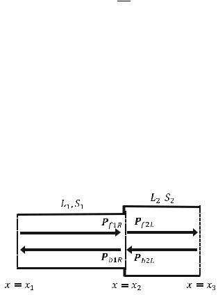
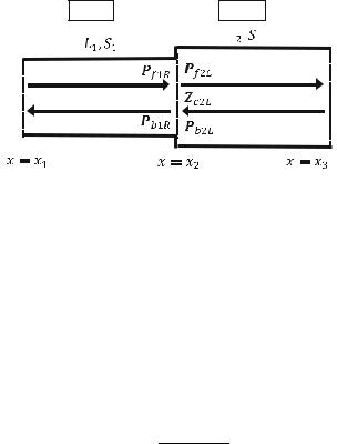
The cross-sectional areas of Pipe 1 and Pipe 2 are S1 and S2, respectively, as shown in the figure below. The pressures of the forward wave and the backward wave in Pipe 1 at RHS of Pipe 1 (x ¼ x2) are Pf1R and Pb1R, respectively. The pressures of the forward wave and the backward wave in Pipe 2 at LHS of Pipe 2 (x ¼ x2) are Pf2L and Pb2L, respectively:
Pipe 2
 ,
, 
The pressures Pf1R and Pb1R (RHS of Pipe 1) can be formulated in terms of the
pressures Pf2L and Pb2L (LHS in Pipe 2) as: |
|
|
|
|
|
|
|
|
|
|
|||||||||||||||||||||
|
1 |
|
Z f 1 |
|
|
|
|
|
|
|
1 |
|
|
|
|
|
Z f 1 |
|
|
|
|
||||||||||
P f 1R ¼ |
|
|
1 þ |
|
|
|
|
|
P f 2L þ |
|
|
|
1 |
|
|
|
|
|
Pb2L |
ðFormula 4A’Þ |
|||||||||||
2 |
Z f 2 |
2 |
Z f 2 |
||||||||||||||||||||||||||||
Pb1R ¼ |
1 |
1 |
Z f 1 |
|
P f 2L þ |
1 |
|
1 |
þ |
Z f 1 |
Pb2L |
ðFormula 4B’Þ |
|||||||||||||||||||
2 |
Z f 2 |
|
|
2 |
|
Z f 2 |
|
|
|||||||||||||||||||||||
|
|
|
1 |
1 þ |
Z f 1 |
|
|
|
|
|
|
|
|
|
|
|
|
|
|||||||||||||
|
|
|
P f 1R ¼ |
|
|
|
|
|
Pc2L |
|
|
|
|
|
|
ðFormula 4AÞ |
|||||||||||||||
|
|
|
2 |
Zc2L |
|
|
|
|
|
|
|
||||||||||||||||||||
|
|
|
|
|
Pb1R ¼ |
1 |
1 |
Z f 1 |
|
|
|
|
|||||||||||||||||||
|
|
|
|
|
|
|
|
Pc2L |
ðFormula 4BÞ |
||||||||||||||||||||||
|
|
|
|
|
2 |
Zc2L |
|||||||||||||||||||||||||
|
|
|
|
|
|
|
|
|
|
Pb1R |
|
|
|
|
|
|
Zc2L Z f 1 |
|
|
|
Formula 4C |
|
|||||||||
|
|
|
|
|
|
|
|
|
|
P f 1R |
¼ |
|
|
|
|
ð |
Þ |
||||||||||||||
|
|
|
|
|
|
|
|
|
|
|
|
Zc2L |
þ |
Z f 1 |
|
|
|||||||||||||||
|
|
|
|
|
|
|
|
|
|
|
|
|
|
|
|
|
|
|
|
|
|
|
|
|
|
|
|
|
|
|
|
|
|
|
|
|
|
|
|
|
|
Pc2L |
|
¼ |
|
|
|
|
|
2Zc2L |
|
ðFormula 4DÞ |
|||||||||||
|
|
|
|
|
|
|
|
|
|
P f 1R |
|
|
|
Zc2L |
þ |
Z f 1 |
|
|
|||||||||||||
|
|
|
|
|
|
|
|
|
|
|
|
|
|
|
|
|
|
|
|
|
|
|
|
|
|
|
|
|
|
|
|
