
- •Preface
- •Objectives of the Book
- •Style
- •Prerequisites
- •The Big Picture
- •Contents
- •1.1 Review of Complex Numbers
- •1.2 Complex Numbers in Polar Form
- •1.3 Four Equivalent Forms to Represent Harmonic Waves
- •1.4 Mathematical Identity
- •1.5 Derivation of Four Equivalent Forms
- •1.5.1 Obtain Form 2 from Form 1
- •1.5.2 Obtain Form 3 from Form 2
- •1.5.3 Obtain Form 4 from Form 3
- •1.6 Visualization and Numerical Validation of Form 1 and Form 2
- •1.8 Homework Exercises
- •1.9 References of Trigonometric Identities
- •1.9.1 Trigonometric Identities of a Single Angle
- •1.9.2 Trigonometric Identities of Two Angles
- •1.10 A MATLAB Code for Visualization of Form 1 and Form 2
- •2.2 Equation of Continuity
- •2.3 Equation of State
- •2.3.1 Energy Increase due to Work Done
- •2.3.2 Pressure due to Colliding of Gases
- •2.3.3 Derivation of Equation of State
- •2.4 Derivation of Acoustic Wave Equation
- •2.5 Formulas for the Speed of Sound
- •2.5.1 Formula Using Pressure
- •2.5.2 Formula Using Bulk Modulus
- •2.5.3 Formula Using Temperature
- •2.5.4 Formula Using Colliding Speed
- •2.6 Homework Exercises
- •3.1 Review of Partial Differential Equations
- •3.1.1 Complex Solutions of a Partial Differential Equation
- •3.1.2 Trigonometric Solutions of a Partial Differential Equation
- •3.2 Four Basic Complex Solutions
- •3.3 Four Basic Traveling Waves
- •3.4 Four Basic Standing Waves
- •3.5 Conversion Between Traveling and Standing Waves
- •3.6 Wavenumber, Angular Frequency, and Wave Speed
- •3.7 Visualization of Acoustic Waves
- •3.7.1 Plotting Traveling Wave
- •3.7.2 Plotting Standing Wave
- •3.8 Homework Exercises
- •4.2 RMS Pressure
- •4.2.1 RMS Pressure of BTW
- •4.2.2 RMS Pressure of BSW
- •4.3 Acoustic Intensity
- •4.3.1 Acoustic Intensity of BTW
- •4.3.2 Acoustic Intensity of BSW
- •4.5.1 Issues with Real Impedance
- •4.6 Computer Program
- •4.7 Homework Exercises
- •4.8 References
- •4.8.1 Derivatives of Trigonometric and Complex Exponential Functions
- •4.8.2 Trigonometric Integrals
- •5.1 Spherical Coordinate System
- •5.2 Wave Equation in Spherical Coordinate System
- •5.3 Pressure Solutions of Wave Equation in Spherical Coordinate System
- •5.4 Flow Velocity
- •5.4.1 Flow Velocity in Real Format
- •5.4.2 Flow Velocity in Complex Format
- •5.5 RMS Pressure and Acoustic Intensity
- •5.7 Homework Exercises
- •6.1 Review of Pressure and Velocity Formulas for Spherical Waves
- •6.2 Acoustic Waves from a Pulsating Sphere
- •6.3 Acoustic Waves from a Small Pulsating Sphere
- •6.4 Acoustic Waves from a Point Source
- •6.4.1 Point Sources Formulated with Source Strength
- •6.4.2 Flow Rate as Source Strength
- •6.5 Acoustic Intensity and Sound Power
- •6.6 Computer Program
- •6.7 Project
- •6.8 Objective
- •6.9 Homework Exercises
- •7.1 1D Standing Waves Between Two Walls
- •7.2 Natural Frequencies and Mode Shapes in a Pipe
- •7.3 2D Boundary Conditions Between Four Walls
- •7.3.1 2D Standing Wave Solutions of the Wave Equation
- •7.3.2 2D Nature Frequencies Between Four Walls
- •7.3.3 2D Mode Shapes Between Four Walls
- •7.4 3D Boundary Conditions of Rectangular Cavities
- •7.4.1 3D Standing Wave Solutions of the Wave Equation
- •7.4.2 3D Natural Frequencies and Mode Shapes
- •7.5 Homework Exercises
- •8.1 2D Traveling Wave Solutions
- •8.1.2 Wavenumber Vectors in 2D Traveling Wave Solutions
- •8.2 Wavenumber Vectors in Resonant Cavities
- •8.3 Traveling Waves in Resonant Cavities
- •8.4 Wavenumber Vectors in Acoustic Waveguides
- •8.5 Traveling Waves in Acoustic Waveguides
- •8.6 Homework Exercises
- •9.1 Decibel Scale
- •9.1.1 Review of Logarithm Rules
- •9.1.2 Levels and Decibel Scale
- •9.1.3 Decibel Arithmetic
- •9.2 Sound Pressure Levels
- •9.2.2 Sound Power Levels and Decibel Scale
- •9.2.3 Sound Pressure Levels and Decibel Scale
- •9.2.4 Sound Pressure Levels Calculated in Time Domain
- •9.2.5 Sound Pressure Level Calculated in Frequency Domain
- •9.3 Octave Bands
- •9.3.1 Center Frequencies and Upper and Lower Bounds of Octave Bands
- •9.3.2 Lower and Upper Bounds of Octave Band and 1/3 Octave Band
- •9.3.3 Preferred Speech Interference Level (PSIL)
- •9.4 Weighted Sound Pressure Level
- •9.4.1 Logarithm of Weighting
- •9.5 Homework Exercises
- •10.1 Sound Power, Acoustic Intensity, and Energy Density
- •10.2.2 Room Constant
- •10.2.3 Reverberation Time
- •10.3 Room Acoustics
- •10.3.1 Energy Density due to an Acoustic Source
- •10.3.2 Sound Pressure Level due to an Acoustic Source
- •10.4 Transmission Loss due to Acoustical Partitions
- •10.4.2 Transmission Loss (TL)
- •10.5 Noise Reduction due to Acoustical Partitions
- •10.5.1 Energy Density due to a Partition Wall
- •10.5.2 Sound Pressure Level due to a Partition Wall
- •10.5.3 Noise Reduction (NR)
- •10.6 Homework Exercises
- •11.1 Complex Amplitude of Pressure and Acoustic Impedance
- •11.1.3 Transfer Pressure
- •11.2 Complex Acoustic Impedance
- •11.3 Balancing Pressure and Conservation of Mass
- •11.4 Transformation of Pressures
- •11.5 Transformation of Acoustic Impedance
- •11.7 Numerical Method for Molding of Pipelines
- •11.8 Computer Program
- •11.9 Project
- •11.10 Homework Exercises
- •12.1.1 Equivalent Acoustic Impedance of a One-to-Two Pipe
- •12.2 Power Transmission of a One-to-Two Pipe
- •12.3 Low-Pass Filters
- •12.4 High-Pass Filters
- •12.5 Band-Stop Resonator
- •12.6 Numerical Method for Modeling of Pipelines with Side Branches
- •12.7 Project
- •12.8 Homework Exercises
- •Nomenclature
- •Appendices
- •Appendix 1: Discrete Fourier Transform
- •Discrete Fourier Transform
- •Fourier Series for Periodical Time Function
- •Formulas of Discrete Fourier Series
- •Appendix 2: Power Spectral Density
- •Power Spectral Density
- •Accumulated Sound Pressure Square
- •Sound Pressure Level in Each Band
- •References
- •Index

9.3 Octave Bands |
237 |
Example 9.4: Solution
(a)The RMS pressure can be formulated in the frequency domain using Parseval’s theorem as:
1 p2RMS ¼ P2o þ 12 X P2k
k¼1
The RMS pressure can be calculated in the frequency domain by substituting the given frequency contents Pk into the equation above:
pRMS2 ¼ Po2 |
þ |
1 |
1 |
Pk2 |
= |
P2 |
= |
32 |
hðPaÞ2i |
2 |
k¼1 |
21 |
2 |
||||||
|
|
|
X |
|
|
|
|
|
|
(b) The unweighted SPL calculated in the frequency domain is:
|
|
3 |
! ½dB& |
|
|
|
|||
Lp ¼ 20 log 10 |
PRMS |
p2 |
||
Pr |
¼ 20 log 10 20 |
10 6 |
Note that both RMS pressure and unweighted SPL calculated in the frequency domain (this example) are the same as if calculated in the time domain (the previous example). This is the expected result because of Parseval’s theorem.
9.3Octave Bands
Octave bands are commonly used in the fields of acoustics and vibration. Two major benefits of using octave bands are as follows: (1) it provides insight of power distribution vs. frequency, and (2) it allows to apply weight to the different frequencies.
9.3.1Center Frequencies and Upper and Lower Bounds of Octave Bands
Spectra obtained by Fourier transform (FT) using frequency in linear scale are called the narrow band spectra. However, such detail in spectral resolution is not always needed. Hence, spectra can be obtained in wider frequency bands for easier analysis. The most commonly used frequency bands are octave bands (frequency in logarithmic scale). Each octave band has a center frequency and a band width, defined as:
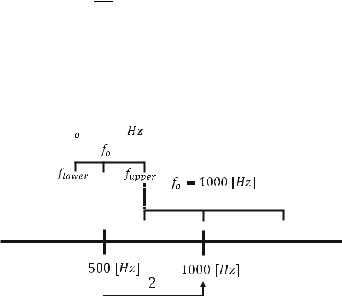
238 |
9 Sound Pressure Levels and Octave Bands |
|
k |
½octave& |
f o ¼ 1000 2 |
1 |
½octave& |
~ |
½center frequency& |
½Hz&; k ¼ 54; |
f lower ¼ |
f o |
¼ f o ∙ 2 |
1 |
; |
½lower limit frequency& |
|
|||||||
p2 |
|
2 |
|
||||||||||
f upper ¼ |
|
|
o ¼ |
|
o ∙ |
|
1 |
|
½ |
|
1 |
& |
|
|
f |
22 |
; |
|
|||||||||
|
p2 f |
|
|
|
|
upper limit frequency |
|
||||||
|
|
|
f upper ¼ f lower ∙ 2 |
|
|
= 500 [ ]
|
center |
lower |
upper |
The center frequencies and lower and upper limit frequencies of octave bands are:
1 Octave |
|
|
|
|
|
|
|
|
|
Band |
|
Center (Quoted) |
|
Center (Quoted) |
Center (Calculated) |
Lower (Limit) |
|
Upper (Limit) |
|
[-] |
|
|
|
[Hz] |
[Hz] |
[Hz] |
[Hz] |
||
|
|
|
|
|
fo |
fo*2^(-1/2) |
|
fo*2^(1/2) |
|
0 |
|
1000*2^(-5) |
|
31.50 |
31.25 |
22.10 |
|
44.19 |
|
1 |
|
1000*2^(-4) |
|
63.00 |
62.50 |
44.19 |
|
88.39 |
|
2 |
|
1000*2^(-3) |
|
125.00 |
125.00 |
88.39 |
|
176.78 |
|
|
|
|
|
|
|
176.78 |
|
353.55 |
|
3 |
|
1000*2^(-2) |
|
250.00 |
250.00 |
|
|
||
|
|
|
|
|
|
353.55 |
|
707.11 |
|
4 |
|
1000*2^(-1) |
|
500.00 |
500.00 |
|
|
||
5 |
|
1000*2^0 |
|
1000.00 |
1000.00 |
707.11 |
|
1414.21 |
|
|
|
|
|
|
|
1414.21 |
|
2828.43 |
|
6 |
|
1000*2^1 |
|
2000.00 |
2000.00 |
|
|
||
7 |
|
1000*2^2 |
|
4000.00 |
4000.00 |
2828.43 |
|
5656.85 |
|
|
|
|
|
|
|
5656.85 |
|
11313.71 |
|
8 |
|
1000*2^3 |
|
8000.00 |
8000.00 |
|
|
||
9 |
|
1000*2^4 |
|
16000.00 |
16000.00 |
11313.71 |
|
22627.42 |
|

9.3 Octave Bands |
239 |
9.3.2Lower and Upper Bounds of Octave Band and 1/3 Octave Band
There are other popular wide bands in the analysis that can use 13 octave bands, 101 octave bands, and 121 octave bands. The formula for 13 octave bands is shown below:
|
k |
½octave& |
f o ¼ 1000 2 |
3 |
½octave& |
~ |
½center frequency& |
½Hz&; k ¼ 1913; |
|
|
f o |
|
|
¼ f o ∙ 2 |
1 |
|
f lower ¼ |
|
|
|
6 |
; |
||
|
p2 |
1=3 |
|||||
f upper ¼ |
|
|
1=3 |
f o ¼ f o ∙ |
1 |
||
p2 |
|
26 |
|||||
|
|
|
|
|
1 |
|
|
f upper ¼ f lower ∙ 23 |
|
|
In general, m-octave bands can be generated using the relationships below:
f o ¼ 1000 ∙ ð2mÞk, where m ¼ 1, 12 , 13 , 14
f lower ¼ 2 m=2 f o; f upper ¼ 2m=2 f o; f upper ¼ 2m f lower
Example 9.6
Given the time domain function p(t) with frequency contents Pk as below:
pðtÞ ¼ X4k¼1Pk cos ð2π f kt þ θkÞ
where:
f k ¼ 250 k ½Hz&
And the magnitudes and phases are:
P1 = 0.023[Pa]; |
θ1 |
= 0 [deg] |
P2 = 0.127[Pa]; |
θ2 |
= 270[deg] |
P3 = 0.127[Pa]; |
θ3 |
= 270[deg] |
P4 = 0.283[Pa]; |
θ3 |
= 270[deg] |
Determine the combined sound pressure level (SPL) using the following three methods:

240 |
9 Sound Pressure Levels and Octave Bands |
(a)Calculate the combined SPL from the summation of the square of the RMS pressures.
(b)Calculate the combined SPL from the SPL spectrum of all the existing frequencies.
(c)Calculate the combined SPL from the SPL spectrum of the octave bands.
Example 9.6: Solution
(a)Calculate the combined SPL from the summation of the square of the RMS pressures.
The RMS pressures of each frequency are:
2 |
|
= |
P12 |
|
|
|
0:0232 |
|
|
2 |
|
||||||
pRMS,250Hz |
|
|
¼ |
|
|
|
|
|
|
|
Pa |
|
2 |
||||
2 |
2 |
2 |
|
|
|
||||||||||||
p2 |
= p2 |
|
|
Hz |
= |
P2 |
|
|
0:127 |
|
Pa2 |
||||||
|
|
|
|
|
|
|
|
|
|
|
|||||||
|
|
|
|
|
|
|
|
|
¼ |
|
|
|
|
|
|
||
RMS,500Hz |
RMS,750 2 |
|
|
|
2 |
2 |
2 |
|
|
||||||||
2 |
|
= |
|
P4 |
|
|
|
0:283 |
|
|
|
|
2 |
|
|||
pRMS,1000Hz |
|
|
|
¼ |
|
|
|
|
|
|
Pa |
|
|
||||
2 |
|
|
|
|
2 |
|
|
|
The combined SPL from the summation of the square of the RMS pressure is:
|
|
|
|
|
|
|
|
|
|
¼ |
|
|
|
|
|
|
|
Pr2 |
|
! |
|
|
|
|
|
|
|
|
||
|
|
|
|
|
|
|
|
|
|
|
|
|
|
|
|
|
|
P2 |
|
|
|
|
|
|
|
|
|
|
||
|
|
|
|
|
|
|
Lp |
|
|
10 log 10 |
|
RMS,total |
|
|
|
|
|
|
|
|
|
|||||||||
|
|
|
|
|
|
|
|
|
|
|
|
|
|
|
|
|
|
|
|
|
|
|||||||||
|
|
|
0 |
: |
0232 |
|
0 |
: |
1272 |
|
0 |
1272 |
|
0: |
2832 |
|
|
|
|
|
|
|
|
|||||||
|
|
|
0 |
|
|
þ |
|
|
|
|
þ |
|
|
: |
|
|
þ |
|
|
|
1 |
|
|
|
|
|
|
|||
¼ |
10 log |
10 |
|
|
2 |
|
|
|
2 |
|
|
|
|
2 |
|
|
2 |
|
|
dB |
& ¼ |
81:495 |
½ |
dB |
& |
|||||
|
|
B |
|
|
|
|
|
|
20 10 6 |
|
|
|
|
|
|
C½ |
|
|
|
|||||||||||
|
|
|
@ |
|
|
|
|
|
|
|
|
|
|
|
|
|
|
|
|
|
|
A |
|
|
|
|
|
|
(b)Calculate the combined SPL from the SPL spectrum of all the existing frequencies:
|
¼ |
|
|
Pr2 |
! |
¼ |
|
|
|
20 10 6 2!½ & ¼ |
½ & |
|||||||
|
|
|
P2 |
|
|
|
|
|
|
|
|
|
0:0232 |
|
|
|
|
|
Lp,250Hz |
|
10 log 10 |
|
RMS, 250Hz |
|
|
10 log 10 |
|
|
2 |
|
|
dB |
58:2037 dB |
||||
|
|
P2 |
! |
|
|
0:1272 |
|
|
||||||||||
|
¼ |
|
¼ |
|
|
|
|
|
½ & |
|||||||||
|
|
Pr2 |
|
|
|
|
20 ∙ 10 6 2!½ & ¼ |
|||||||||||
Lp,500Hz |
|
10 log 10 |
|
RMS,500Hz |
|
|
|
|
10 log 10 |
|
|
2 |
|
|
dB |
73:0452 dB |
||
|
|
|
|
|
|
|
|
|
|
|||||||||
|
|
|
|
|
L |
p,750Hz ¼ |
L |
|
|
|
|
|||||||
|
|
|
|
|
|
|
|
p,500Hz |
|
|
|
|
||||||
|
|
|
2 |
|
|
|
|
|
|
|
|
|
0:2832 |
|
|
!½dB& ¼ 80:0048½dB& |
||
|
|
|
|
P |
|
|
|
|
|
|
|
|
|
2 |
|
|
||
|
|
|
|
RMS,1000Hz |
|
|
|
|
|
|
|
|
|
|||||
Lp,1000Hz ¼ 10 log 10 |
|
|
|
! ¼ 10 log 10 |
|
|
20 ∙ 10 6 |
|
2 |
|||||||||
|
Pr2 |
|
|
|
||||||||||||||
|
|
|
|
|
|
|
|
|
|
|
|
|
|
|
|