
- •Preface
- •Objectives of the Book
- •Style
- •Prerequisites
- •The Big Picture
- •Contents
- •1.1 Review of Complex Numbers
- •1.2 Complex Numbers in Polar Form
- •1.3 Four Equivalent Forms to Represent Harmonic Waves
- •1.4 Mathematical Identity
- •1.5 Derivation of Four Equivalent Forms
- •1.5.1 Obtain Form 2 from Form 1
- •1.5.2 Obtain Form 3 from Form 2
- •1.5.3 Obtain Form 4 from Form 3
- •1.6 Visualization and Numerical Validation of Form 1 and Form 2
- •1.8 Homework Exercises
- •1.9 References of Trigonometric Identities
- •1.9.1 Trigonometric Identities of a Single Angle
- •1.9.2 Trigonometric Identities of Two Angles
- •1.10 A MATLAB Code for Visualization of Form 1 and Form 2
- •2.2 Equation of Continuity
- •2.3 Equation of State
- •2.3.1 Energy Increase due to Work Done
- •2.3.2 Pressure due to Colliding of Gases
- •2.3.3 Derivation of Equation of State
- •2.4 Derivation of Acoustic Wave Equation
- •2.5 Formulas for the Speed of Sound
- •2.5.1 Formula Using Pressure
- •2.5.2 Formula Using Bulk Modulus
- •2.5.3 Formula Using Temperature
- •2.5.4 Formula Using Colliding Speed
- •2.6 Homework Exercises
- •3.1 Review of Partial Differential Equations
- •3.1.1 Complex Solutions of a Partial Differential Equation
- •3.1.2 Trigonometric Solutions of a Partial Differential Equation
- •3.2 Four Basic Complex Solutions
- •3.3 Four Basic Traveling Waves
- •3.4 Four Basic Standing Waves
- •3.5 Conversion Between Traveling and Standing Waves
- •3.6 Wavenumber, Angular Frequency, and Wave Speed
- •3.7 Visualization of Acoustic Waves
- •3.7.1 Plotting Traveling Wave
- •3.7.2 Plotting Standing Wave
- •3.8 Homework Exercises
- •4.2 RMS Pressure
- •4.2.1 RMS Pressure of BTW
- •4.2.2 RMS Pressure of BSW
- •4.3 Acoustic Intensity
- •4.3.1 Acoustic Intensity of BTW
- •4.3.2 Acoustic Intensity of BSW
- •4.5.1 Issues with Real Impedance
- •4.6 Computer Program
- •4.7 Homework Exercises
- •4.8 References
- •4.8.1 Derivatives of Trigonometric and Complex Exponential Functions
- •4.8.2 Trigonometric Integrals
- •5.1 Spherical Coordinate System
- •5.2 Wave Equation in Spherical Coordinate System
- •5.3 Pressure Solutions of Wave Equation in Spherical Coordinate System
- •5.4 Flow Velocity
- •5.4.1 Flow Velocity in Real Format
- •5.4.2 Flow Velocity in Complex Format
- •5.5 RMS Pressure and Acoustic Intensity
- •5.7 Homework Exercises
- •6.1 Review of Pressure and Velocity Formulas for Spherical Waves
- •6.2 Acoustic Waves from a Pulsating Sphere
- •6.3 Acoustic Waves from a Small Pulsating Sphere
- •6.4 Acoustic Waves from a Point Source
- •6.4.1 Point Sources Formulated with Source Strength
- •6.4.2 Flow Rate as Source Strength
- •6.5 Acoustic Intensity and Sound Power
- •6.6 Computer Program
- •6.7 Project
- •6.8 Objective
- •6.9 Homework Exercises
- •7.1 1D Standing Waves Between Two Walls
- •7.2 Natural Frequencies and Mode Shapes in a Pipe
- •7.3 2D Boundary Conditions Between Four Walls
- •7.3.1 2D Standing Wave Solutions of the Wave Equation
- •7.3.2 2D Nature Frequencies Between Four Walls
- •7.3.3 2D Mode Shapes Between Four Walls
- •7.4 3D Boundary Conditions of Rectangular Cavities
- •7.4.1 3D Standing Wave Solutions of the Wave Equation
- •7.4.2 3D Natural Frequencies and Mode Shapes
- •7.5 Homework Exercises
- •8.1 2D Traveling Wave Solutions
- •8.1.2 Wavenumber Vectors in 2D Traveling Wave Solutions
- •8.2 Wavenumber Vectors in Resonant Cavities
- •8.3 Traveling Waves in Resonant Cavities
- •8.4 Wavenumber Vectors in Acoustic Waveguides
- •8.5 Traveling Waves in Acoustic Waveguides
- •8.6 Homework Exercises
- •9.1 Decibel Scale
- •9.1.1 Review of Logarithm Rules
- •9.1.2 Levels and Decibel Scale
- •9.1.3 Decibel Arithmetic
- •9.2 Sound Pressure Levels
- •9.2.2 Sound Power Levels and Decibel Scale
- •9.2.3 Sound Pressure Levels and Decibel Scale
- •9.2.4 Sound Pressure Levels Calculated in Time Domain
- •9.2.5 Sound Pressure Level Calculated in Frequency Domain
- •9.3 Octave Bands
- •9.3.1 Center Frequencies and Upper and Lower Bounds of Octave Bands
- •9.3.2 Lower and Upper Bounds of Octave Band and 1/3 Octave Band
- •9.3.3 Preferred Speech Interference Level (PSIL)
- •9.4 Weighted Sound Pressure Level
- •9.4.1 Logarithm of Weighting
- •9.5 Homework Exercises
- •10.1 Sound Power, Acoustic Intensity, and Energy Density
- •10.2.2 Room Constant
- •10.2.3 Reverberation Time
- •10.3 Room Acoustics
- •10.3.1 Energy Density due to an Acoustic Source
- •10.3.2 Sound Pressure Level due to an Acoustic Source
- •10.4 Transmission Loss due to Acoustical Partitions
- •10.4.2 Transmission Loss (TL)
- •10.5 Noise Reduction due to Acoustical Partitions
- •10.5.1 Energy Density due to a Partition Wall
- •10.5.2 Sound Pressure Level due to a Partition Wall
- •10.5.3 Noise Reduction (NR)
- •10.6 Homework Exercises
- •11.1 Complex Amplitude of Pressure and Acoustic Impedance
- •11.1.3 Transfer Pressure
- •11.2 Complex Acoustic Impedance
- •11.3 Balancing Pressure and Conservation of Mass
- •11.4 Transformation of Pressures
- •11.5 Transformation of Acoustic Impedance
- •11.7 Numerical Method for Molding of Pipelines
- •11.8 Computer Program
- •11.9 Project
- •11.10 Homework Exercises
- •12.1.1 Equivalent Acoustic Impedance of a One-to-Two Pipe
- •12.2 Power Transmission of a One-to-Two Pipe
- •12.3 Low-Pass Filters
- •12.4 High-Pass Filters
- •12.5 Band-Stop Resonator
- •12.6 Numerical Method for Modeling of Pipelines with Side Branches
- •12.7 Project
- •12.8 Homework Exercises
- •Nomenclature
- •Appendices
- •Appendix 1: Discrete Fourier Transform
- •Discrete Fourier Transform
- •Fourier Series for Periodical Time Function
- •Formulas of Discrete Fourier Series
- •Appendix 2: Power Spectral Density
- •Power Spectral Density
- •Accumulated Sound Pressure Square
- •Sound Pressure Level in Each Band
- •References
- •Index

8.1 2D Traveling Wave Solutions |
199 |
Based on the formulas shown above, topics such as cutoff frequency, echoes, and sound distortion in waveguides will be discussed in this chapter.
8.12D Traveling Wave Solutions
8.1.1Definition of Wavenumber Vectors
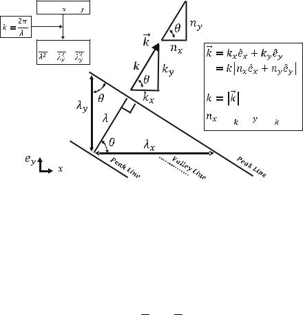
We have derived the relationship between the combined wavenumber k and the component wavenumbers kx and ky in Chap. 7:
k2 ¼ k2x þ k2y
Substituting the relationship between the wavenumber k and the wavelength λ:
2π k ¼ λ
into the first equation gives the relationship between the combined wavelength λ and the component wavelengths λx and λy as:
1 ¼ 1 þ 1
λ2 λ2x λ2y
The relationship above can also be proved geometrically with trigonometric relationships:
cos θ ¼ |
λ |
; sin θ ¼ |
|
λ |
|
|
|
|
|
|
||||
λx |
λy |
|
|
|
|
|
|
|
||||||
and the trigonometric identity: |
|
|
|
|
|
|
|
|
|
|
|
|
|
|
cos 2θ þ sin 2θ ¼ 1 ! 1 |
¼ |
λ2 |
þ |
λ2 |
! |
1 |
¼ |
1 |
þ |
1 |
||||
λ2 |
λ2 |
λ2 |
|
λ2 |
λ2 |
|||||||||
|
|
|
x |
|
y |
|
|
|
|
|
x |
|
y |

200 |
8 Acoustic Waveguides |
=
+
1
1 = 1 + 1
Where
= ;
=
̂
̂
The combined wavenumber is a vector that presents the propagation direction and the magnitude of a 2D propagating plane wave as:
!
k¼ kxbex þ kybey
¼k nxbex þ nybey
where:
nx ¼ kkx ; ny ¼ kky
where bex and bey are the base vectors of the Cartesian coordinate systems and kx and ky
!
are vector components of k .
!
Note that nx and ny indicate the direction of the wavenumber vector k and have the following properties:
nx ¼ cos θ; ny ¼ sin θ
! n2x þ n2y ¼ 1

8.1 2D Traveling Wave Solutions |
201 |
8.1.2Wavenumber Vectors in 2D Traveling Wave Solutions
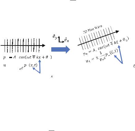
The sound pressure and flow velocity of 1D plane waves were derived in Chap. 4 and are listed below for reference:
p ðx, tÞ ¼ A cos ðωt kx þ θ Þ
1
u ðx, tÞ ¼ ρoc p ðx, tÞ
The formulas above will be transferred to 2D plane waves using the wavenumber vector we learned in the previous section:
1D Plan Wave
± |
± |
± |
|
|
|||
± = ± |
1 |
|
|
|
|||
± |
|
A single variable |
|||||
ρ |
|||||||
|
|
|
|
|
|
||
|
|
|
|
|
|
||
|
|
|
|
|
|
|
|
|
|
|
|
A single variable |
|
|
|
|
|
|
|
|
|
|
Note that the formulas of pressure and velocity on the left-hand side of the figure are for the plane wave traveling along the x-axis. The right-hand side of the figure shows the same plane wave rotated by an angle. The rotated plane wave becomes 2D and can be formulated with a new variable ξ. The formulas of pressure and velocity of the 2D plane wave are the same as the 1D plane wave except using the different variable names – x and ξ as:
p ðξ, tÞ ¼ A cos ðωt kξ þ θ Þ
1
u ðξ, tÞ ¼ ρoc p ðξ, tÞ along traveling direction
The new variable ξ is the result of the dot product of the wavenumber vector
! !
k kx, ky and the position vector r ðx, yÞ as:
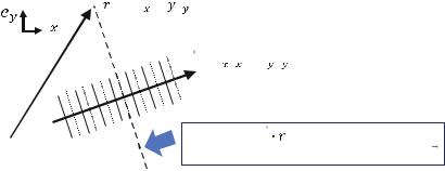
202 |
|
|
|
|
|
|
|
|
|
|
|
|
|
8 |
|
Acoustic Waveguides |
|||
|
! |
! |
|
|
|
|
|
|
|
|
|
|
|
|
|
|
|
|
|
ξ ¼ |
|
k ∙ |
r |
|
|
|
|
|
|
|
|
|
|
|
|
|
|
|
|
|
!k |
|
|
|
|
|
|
|
|
|
|
|
|
|
|
|
|
||
|
|
|
|
|
ð |
|
Þ |
|
|
þ |
|
|
|
|
k |
|
|
||
|
|
kx |
, ky |
|
∙ |
x, y |
|
kxx |
kyy |
|
kxx |
þ |
kyy |
||||||
|
|
|
|
|
|
|
|
|
|
q |
|
|
|
|
|
|
|||
¼ |
|
|
|
! |
|
|
|
|
¼ |
¼ |
|
|
|
|
|
||||
|
|
|
|
k |
|
|
|
|
|
kx þ ky |
|
|
|
|
|
|
|||
|
|
|
|
|
|
|
|
|
|
|
|
|
|
|
|
||||
¼ |
nxx |
þ |
|
|
|
|
|
|
|
|
|
|
|
|
|||||
|
|
nyy |
|
|
|
|
|
|
|
|
|
|
|
|
!
And the velocity of the plane wave above is along the traveling direction k :
̂= ̂+
̂
̂
̂
̂
The value of is the same on a plane that is perpendicular to the wavenumber vector
Based on the formulas above, the pressure and velocity of a 2D plane wave can be formulated in the Cartesian coordinate as:
p ðx, y, tÞ ¼ A cos ðωt kξ þ θ Þ |
|
||||||
¼ A cos |
ωt k nxx þ nyy þ θ |
||||||
¼ A cos |
ωt kxx þ kyy |
þ θ |
|||||
¼ A cos hωt !k ∙ !r þ θ i |
|||||||
where: |
!k |
|
|||||
k ¼ |
|
||||||
kx |
|
ky |
|
||||
nx ¼ |
|
; ny ¼ |
|
|
|
||
k |
k |
|
! ’
The 2D flow velocity u of the 2D plane wave can be derived using Euler s force equation as the following:

8.1 2D Traveling Wave Solutions |
|
|
Z |
|
|
|
|
|
|
|
|
|
203 |
||
|
ð |
|
Þ ¼ ρo |
|
½ |
|
ð |
|
|
|
|
Þ& |
|
|
|
!u |
|
x, y, t |
1 |
b |
|
p |
b |
x, y, t |
|
dt |
Þ |
||||
|
|
|
¼ |
|
ρ0c |
|
|
ð |
|
|
|
||||
|
|
|
|
nxex |
þ nyey |
p |
|
x, y, t |
|
||||||
|
|
|
|
|
|
|
|
|
|||||||
|
|
|
|
|
|
|
|
|
|
!
Note that the sound pressure p is a scalar but the flow velocity u is a vector because of the gradient operator .
!
The detailed derivation of the backward flow velocity u 2 is shown in Example
!
8.1. The derivation of the forward flow velocity u þ is one of the homework problems.
Example 8.1: (Derivation of 2D Plane Traveling Waves: Backward)
!
Derive the 2D backward flow velocity vector u ðx, y, tÞ of a 2D plane backward traveling wave from the 2D acoustic pressure p (x, y, t) using Euler’s force equation:
p ðx, y, tÞ ¼ A cos |
ωt þ |
kxx þ kyy þ θ |
|||||||
|
ð |
|
Þ ¼ |
|
b 0 |
b |
ð |
|
Þ |
!u |
|
x, y, t |
|
nxex þ nyey |
p |
x, y, t |
|
||
ρ c |
|
where:
nx
Euler’s force equation:
Example 8.1: Solution
|
kx |
, and ny ¼ |
ky |
|||
¼ |
q |
q |
||||
kx2 þ ky2 |
kx2 þ ky2 |
|||||
pðx, y, tÞ ¼ ρo |
∂ |
! |
ðx, y, tÞ |
|||
∂t |
u |
!
Backward flow velocity u ðx, y, tÞ is a vector and can be calculated from acoustic pressure based on Euler’s force equation:
pðx,
!
! uðx, y,
y, tÞ ¼ ρo |
|
∂ ! |
ðx, y, tÞ |
||
|
u |
||||
∂t |
|||||
tÞ ¼ ρo |
Z |
½ pðx, y, tÞ&dt |
|||
1 |
|
|
|
|
|
Euler’s force equation for the 2D wave equation in Cartesian coordinate is formatted as:
!uðx, y, tÞ ¼ ρo |
Z ex ∂x |
þ ey ∂y pðx, y, tÞ dt |
||
1 |
b |
∂ |
b |
∂ |
|
|
|
Remarks

204 |
8 Acoustic Waveguides |
• Euler’s force equation is valid for both forward and backward waves.
!
• Pressure p(x, y, t) is a scalar function and velocity uðx, y, tÞ is a vector function. Therefore, the backward velocity can be calculated from pressure as:
!u 2 |
ðx, y, tÞ ¼ ρo |
Z |
ex ∂x |
þ ey ∂y p ðx, y, tÞ dt |
|
|
|
|
|
||||||||||||||||
|
|
1 |
|
|
|
b |
∂ |
|
b |
∂ |
|
|
|
|
|
|
|
|
|
|
|
|
|
||
|
¼ ρo Z |
|
|
|
|
|
|
e |
|
Z |
∂y p ðx, y, tÞ dt |
|
|||||||||||||
|
∂x p ðx, y, tÞ dt |
ρo |
|
||||||||||||||||||||||
|
|
|
ex |
|
|
∂ |
|
|
|
|
|
|
|
y |
|
|
∂ |
|
|
|
|
|
|||
|
|
|
b |
|
|
|
|
|
|
|
|
|
|
|
b |
|
|
|
|
|
|
|
|
|
|
Separate the velocity vector |
|
into two |
vector |
components, |
bex |
u |
x ð |
x, y, t |
Þ |
||||||||||||||||
and eyuy ðx, y, tÞ: |
|
|
|
|
|
|
|
|
|
|
|
|
|
|
|
|
|
|
|
|
|
|
|||
b |
|
|
|
|
|
|
|
|
|
|
|
|
|
|
|
|
|
|
|
|
|
|
|
|
|
where:
ux ðx, y,
uy ðx, y,
∂
∂x
!
u ðx, y, tÞ ¼ bexux ðx, y, tÞ þ beyuy ðx, y, tÞ
tÞ ¼ ρo |
Z ∂x p ðx, y, tÞ dt ¼ ρoω p ðx, y, tÞ |
|||
1 |
|
∂ |
|
kx |
tÞ ¼ ρo |
Z ∂y p ðx, y, tÞ dt ¼ ρoω p ðx, y, tÞ |
|||
1 |
|
∂ |
|
ky |
p ðx, y, tÞ ¼ A cos ωt þ |
kxx þ kyy þ θ |
p ðx, y, tÞ ¼ A ∂x cos ωt þ kxx þ kyy |
þ θ |
|
|
∂ |
|
¼ A kx sin ωt þ kxx þ kyy þ θ
8.1 2D Traveling Wave Solutions |
|
|
|
|
|
|
|
|
|
|
|
|
|
|
|
|
|
|
|
|
|
|
|
|
|
|
205 |
||||
|
|
|
|
|
|
|
|
|
|
|
|
|
|
∂ |
|
|
|
|
|
|
|
|
|
|
|
|
|
|
|
|
|
|
ux ðx, y, tÞ ¼ Z |
|
p ðx, y, tÞ dt |
|
|
|
|
|
|
|
|
|
|||||||||||||||||||
|
∂x |
|
|
|
|
|
|
|
|
|
|||||||||||||||||||||
|
¼ A kx Z sin ωt þ kxx þ kyy þ θ dt |
|
|
|
|
|
|
|
|
||||||||||||||||||||||
|
¼ A ω cos ωt þ kxx þ kyy þ θ |
|
|
|
|
|
|
|
|
||||||||||||||||||||||
|
|
|
|
kx |
|
|
|
|
|
|
|
|
|
|
|
|
|
|
|
|
|
|
|
|
|
|
|
|
|
|
|
|
|
|
|
|
¼ |
ω p ðx, y, tÞ |
|
|
|
|
|
|
|
|
|
|
|
|
|
||||||||||||
|
|
|
|
|
|
|
|
|
kx |
|
|
|
|
|
|
|
|
|
|
|
|
|
|
|
|
|
|
|
|
|
|
Similarly: |
|
|
|
|
|
|
|
|
|
|
|
|
|
|
|
|
|
|
|
|
|
|
|
|
|
|
|
|
|
|
|
uy ðx, y, tÞ ¼ Z ∂y p ðx, y, tÞ dt ¼ ω |
|
|
|
|
|
|
|
|
|
|
|||||||||||||||||||||
|
|
p ðx, y, tÞ |
|
|
|||||||||||||||||||||||||||
|
|
|
|
|
|
|
∂ |
|
|
|
|
|
|
|
|
|
|
|
|
ky |
|
|
|
|
|
|
|
|
|
||
Combining two vector components back to one velocity vector yields |
|
|
|||||||||||||||||||||||||||||
! |
|
|
|
|
|
|
|
|
|
|
|
|
|
|
|
|
|
|
|
|
|
|
|
|
|
|
|
|
|
|
|
u ðx, y, tÞ ¼ exux ðx, y, tÞ þ eyuy ðx, y, tÞ |
ω p x, |
|
|
t |
|
|
|
|
|||||||||||||||||||||||
|
b e x |
|
ω p b |
t ey |
|
|
|
|
|
|
|||||||||||||||||||||
|
¼ b 1 |
kx |
|
|
ð |
x, y, |
Þ b |
|
ky |
|
|
ð |
|
y, |
|
Þ |
|
|
|
||||||||||||
|
ρo |
|
|
|
|
|
ρo |
|
|
|
|
|
|
|
|
|
|||||||||||||||
|
¼ ρoω |
kxex |
þ kyey p ðx, y, tÞ |
|
|
|
|
|
|
|
|
|
|
|
|
|
|||||||||||||||
|
|
|
|
|
|
|
b |
|
|
|
|
b |
|
|
|
|
|
|
|
|
|
|
|
|
|
|
|
7 |
|
|
|
|
|
ρo |
|
|
q6 |
kx |
|
ky |
|
|
|
kx |
|
|
ky |
ð |
Þ |
||||||||||||||
|
|
1 |
|
|
2 |
|
|
|
2 |
2 |
|
|
kx |
|
|
|
|
|
|
ky |
|
|
|
|
3 |
|
x, y, t |
||||
|
¼ ω |
|
kx þ ky |
4q b |
þ |
q b |
5 |
|
|||||||||||||||||||||||
|
|
|
|
2 |
þ |
2 ex |
|
|
2 |
þ |
|
2 ey |
p |
||||||||||||||||||
|
¼ ρo |
|
|
|
|
|
|
|
|
|
|
|
|
|
|
|
|
|
|
|
|
|
|
|
|
|
|
||||
|
ω nxex þ nyey p ðx, y, tÞ |
|
|
|
|
|
|
|
|
|
|
|
|
|
|||||||||||||||||
|
|
k |
|
|
b |
|
|
|
|
b |
|
|
|
|
|
|
|
|
|
|
|
|
|
|
|
|
|
|
|||
where: |
|
|
|
|
|
|
|
|
|
|
|
|
|
|
|
|
|
|
|
|
|
|
|
|
|
|
|
|
|||
|
|
|
|
|
|
|
|
|
|
¼ q |
|
|
|
|
|
|
|
|
|
|
|
|
|
||||||||
|
|
|
|
|
|
|
|
! |
|
|
|
|
|
|
|
|
|
|
|
|
|
||||||||||
|
|
|
|
|
|
|
|
|
|
|
|
|
2 |
|
2 |
|
|
|
|
|
|
|
|
|
|
|
|
|
|
||
|
|
|
|
|
|
kx |
k |
|
|
|
|
|
|
|
|
ky |
|
|
|
|
|
|
|
|
|
|
|
||||
|
|
|
|
|
k |
|
|
|
|
|
kx þ ky |
|
|
|
|
|
|
|
|
|
|
|
|
|
|||||||
|
nx ¼ |
q |
, and ny ¼ |
q |
|
|
|
|
|
|
|
|
|
||||||||||||||||||
|
|
|
kx2 þ ky2 |
|
kx2 þ ky2 |
|
|
|
|
|
|
|
|
|
Replacing ω and k with c yields the final form: