192 7 Resonant Cavities

1

pRMS ¼ p jAj

2

Solve for Plmn using the given RMS pressure ( pRMS ¼ 1 [Pa]) and the location

7.5Homework Exercises

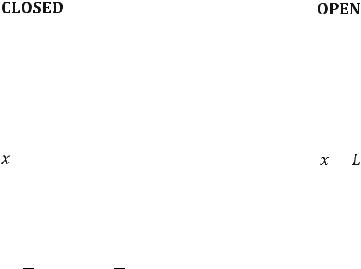
Exercise 7.1 (OPEN-CLOSED PIPE)

A pipe with OPEN-CLOSED boundary conditions has a finite length L as shown below. Set the left end of the pipe as x ¼ 0:

(a)Show that the formulas for the wavenumber and natural frequency of the eigenmode l are:

π

kl ¼ 2L ð2l 1Þ

c

f l ¼ 4L ð2l 1Þ

(b) If L ¼ 0.5 [m],determine the first three natural frequencies, and plot their corresponding mode shapes. Use 340 [m/s] for the speed of sound.

Use 340 [m/s] for the speed of sound (c) in air. Show units in the Meter- Kilogram-Second (MKS) system.

(Answers) (b) 170 [Hz], 510 [Hz], 850 [Hz]

Exercise 7.2 (CLOSE-OPEN PIPE)

A pipe with OPEN-CLOSED boundary conditions has a finite length L as shown below. Set the left end of the pipe as x ¼ 0:

(a)Show that the formulas for the wavenumber and natural frequency of the eigenmode l are:

kl ¼ 2πL ð2l 1Þ, f l ¼ 4cL ð2l 1Þ

(b)If L ¼ 0.5 [m],determine the first three natural frequencies, and plot their corresponding mode shapes. Use 340 [m/s] for the speed of sound.

Use 340 [m/s] for the speed of sound (c) in air. Show units in the Meter- Kilogram-Second (MKS) system.

(Answers) (b) 170 [Hz], 510 [Hz], 850 [Hz]

Exercise 7.3 (3D Rectangular Cavity)

The dimensions of a rectangular cavity are (Lx, Ly, Lz) ¼ (2, 5, 10)[m].

(a)Calculate all resonant frequencies of this cavity that are lower than 60 Hz.

(b)Plot the mode shape of the eigenmode (l, m, n) ¼ (0, 3, 5) using the pressure nodal lines, and indicate the peaks and valleys with “+” and “-” signs, respectively.

(c)Plot the mode shape of the eigenmode (l, m, n) ¼ (0, 5, 8) using the pressure nodal lines, and indicate the peaks and valleys with “+” and “-” signs, respectively.

Use 340 [m/s] for the speed of sound (c) in air. Show units in the Meter- Kilogram-Second (MKS) system.

(Answers): (a) 17 [Hz], 34 [Hz], 38.01 [Hz], 48.08 [Hz], 51 [Hz]

Exercise 7.4 (3D Rectangular Cavity)

The dimensions of a rectangular cavity are (Lx, Ly, Lz) ¼ (3, 4, 10)[m].

(a)Calculate all resonant frequencies of this cavity that are lower than 50 [Hz].

(b)Plot the mode shape of the eigenmode (l, m, n) ¼ (0, 2, 3) using the pressure nodal lines, and indicate the peaks and valleys with “+” and “-” signs, respectively.

(c)Plot the mode shape of the eigenmode (l, m, n) ¼ (0, 5, 8) using the pressure nodal lines, and indicate the peaks and valleys with “+” and “-” signs, respectively.

Use 340 [m/s] for the speed of sound (c) in air. Show units in the Meter- Kilogram-Second (MKS) system.

(Answers): (a) 17 [Hz], 34 [Hz], 42.5 [Hz], 45.8 [Hz]

Exercise 7.5 (3D Rectangular Cavity)

The dimensions of a rectangular cavity are (Lx, Ly, Lz) ¼ (4, 6, 10)[m]. Use 340 [m/s] for the speed of sound.

(a)Calculate the three lowest resonant frequencies of this cavity. Indicate the eigenmode. State the mode numbers.

(b)Plot the mode shape of the eigenmode (l, m, n) ¼ (0, 3, 5) using the pressure nodal lines, and indicate the peaks and valleys with “+” and “-” signs, respectively.

(Answer): (a) f001 ¼ 17 [Hz]; f010 ¼ 28.33 [Hz]; f011 ¼ 33.04 [Hz]

Exercise 7.6 (Standing Waves, Complex) (Optional)

!

Derive the 2D velocity vector usðx, y, tÞ of the plane standing wave from the 2D acoustic pressure using Euler’s force equation. Use complex number format in the derivation:

∙ e jðkxxþθxÞ þ e jðkxxþθxÞ ∙ e jðkyyþθyÞ þ e jðkyyþθyÞ

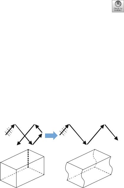
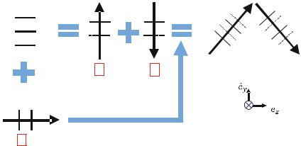
The propagation of plane waves in acoustic waveguides is in the form of resonance (standing waves in the transverse direction) and propagation (traveling waves in the axial direction). Based on what we learned from the previous chapters, we can treat a standing wave (shown in the upper left of the figure below) as the addition of two traveling waves with the same amplitudes and traveling in opposite directions. By adding these two traveling waves (in the transverse direction) back to the traveling wave (in the axial direction), we can reconstruct the propagating wave in the acoustic waveguide as shown in the upper right of the figure below:

After the two walls in the z-direction are removed, the four wavenumber vectors (in 2D resonant cavities as shown in the previous chapter) become two wavenumber vectors because there is no reflection in the z-direction as shown in the figure above. Without the two walls in the z-direction, the wavenumbers in the y-direction are still discretized (as in 2D resonant cavities), but the wavenumbers in the z-direction become continuous numbers as:

In a waveguide, because Lz can be considered as a very large number, and based on the formula above, kzn is continuous. The formulas shown above are the most important formulas of this chapter and will be derived in detail in this chapter.