5.1Spherical Coordinate System

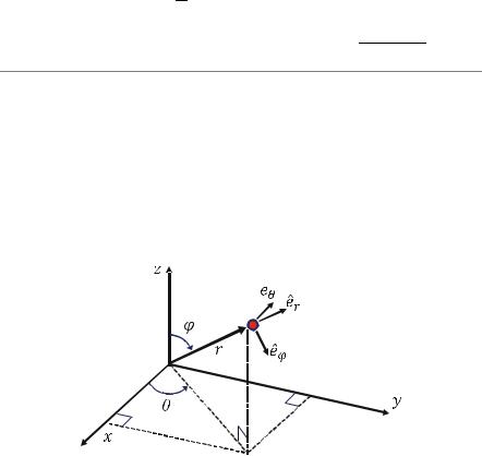
Spherical coordinates consist of three coordinates: r, θ, and φ. These denote the direct distance to a point in space, the lateral angle, and the vertical angle to get there. These three coordinates describe a point in 3D space, just as do three Cartesian coordinates x, y, and z.

The geometry of the spherical coordinates is defined below:

̂

Definition of the coordinates in spherical coordinates

When a vector is expressed in vector format, this expression is independent of the choice of the coordinate systems. A vector can be formulated in the Cartesian coordinates and the spherical coordinates as follows:

Gradient operator is also independent of the choice of coordinate systems. The gradient operator can also be formulated in the Cartesian coordinates and the spherical coordinates as follows:

When the acoustic field is independent of θ and φ, the gradient operator

The Laplacian operator 2 can be formulated in both coordinate systems as:

When the acoustic field is independent of θ and φ, the Laplacian operator simplifies to:

5.2Wave Equation in Spherical Coordinate System

The acoustic wave equation can be formulated in the vector format as:

where the Laplacian operator for Cartesian coordinate and spherical coordinate is shown in the previous section. Because the vector format is independent of the choice of coordinate system, the Laplacian operator, 2, in the equation above can be formulated in both the spherical and Cartesian coordinate systems as shown in the previous section. The one-dimensional wave equation in the spherical coordinate

system can be obtained by replacing the Laplacian operator in vector format in the wave equations as:

The one-dimensional acoustic wave equation in the spherical coordinate system is a function of r and t. The wave equation above can be transferred to the form of the wave equation in the Cartesian coordinate system by defining a new function ϕ(r, t):

ψðr, tÞ rpðr, tÞ

By replacing p(r, t) in the above wave equation with ψ(r, t)/r, the wave equation becomes:

By comparing the wave equations in the spherical coordinate above to the wave equation in the Cartesian coordinate as shown below:

We can see that the wave equation in the spherical coordinate is the same as the wave equation in the Cartesian coordinate. Therefore, the solutions, p(x, t), of the wave equation in the Cartesian coordinate, derived in Chap. 2, can be used as the solutions, ψ(r, t), of the wave equation in the spherical coordinate.

Example 5.1

Show that the following two equations are the same:

Example 5.1 Solution

The Left-Hand Side

The left-hand side of the first equation becomes:

Unlike plane waves, it is hard and unusual to create a symmetrical spherical backward or inward traveling wave. Therefore, only the forward or outward spherical waves are discussed in this course.

The following proves the outward traveling wave solution above. The wave equation in a spherically symmetric pressure field is described as:

∂2p þ 2 ∂p ¼ 1 ∂2p

∂r2 r ∂r c2 ∂t2

The spherical wave equation above can be modified and arranged into the same form as the wave equation for a plane wave. For this purpose, we will define a new function φ:

ψðr, tÞ rpðr, tÞ

Note that ψ could be either a real or a complex number, depending on the equation in which it is used. For example, if ψ is used in a complex equation, it is a complex number. Similarly, if it is used in a real equation, it is a real number.

Substituting the function ψ(r, t) into the following equation will yield the spherical wave equation. The algebra is straightforward and is not shown here, but will be assigned as an exercise:

∂2 ψðr, tÞ ¼ 1 ∂2 ψðr, tÞ

∂r2 c2 ∂t2

Since the above equation has the same form as the one-dimensional plane wave equation, it has the same solutions as shown below:

ψðr, tÞ ¼ ½A c cos ðωt þ krÞ A s sin ðωt þ krÞ&

þ½Aþc cos ðωt krÞ Aþs sin ðωt krÞ& ðRIPÞ

¼ Aþ cos ðωt kr þ θþÞ þ A cos ðωt þ kr þ θ Þ ðREPÞ

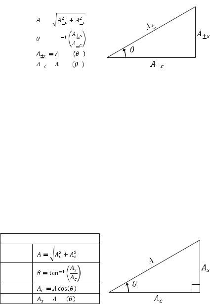
where A , A+, A c, A+c, A s, A+s, θ , and θ+ are real constants related by the following geometry relationships:

Since only forward traveling wave is considered in the spherical coordinates, the above equation can be simplified by defining the following new variables:

Ac Aþc

As Aþs

A Aþ

θ θþ

Therefore, the outward traveling wave in spherical coordinates becomes:

where A, Ac, As, and θ are real variables related by the following geometric relationships:

Geometric Relationship

Geom 1

Transforming the new variable ψ(r, t) back to its original form of pressure p(r, t) yields: