

54 |
|
|
|
|
|
|
|
|
|
|
|
|
|
|
|
|
|
|
|
|
|
|
|
|
|
|
3 Solutions of Acoustic Wave Equation |
||||||||||||||
|
∂2 |
∂ |
|
|
∂ |
|
|
|
|
|
|
|
|
|
∂ |
|
|
∂ |
|
|
|
||||||||||||||||||||
|
|
|
p ¼ |
|
|
|
|
|
|
|
½A s sin ðωt þ kxÞ& |
|
¼ A s |
|
|
½ sin ðωt þ kxÞ& |
|||||||||||||||||||||||||
|
∂x2 |
∂x |
∂x |
∂x |
∂x |
||||||||||||||||||||||||||||||||||||
|
|
|
|
|
|
|
|
|
|
|
∂ |
|
|
|
|
|
|
|
|
|
|
|
|
|
|
|
|
|
|
|
|||||||||||
¼ |
|
A s |
|
|
|
|
fk½ cos ðωt þ kxÞ&g ¼ A sk2 sin ðωt þ kxÞ |
|
|
|
|||||||||||||||||||||||||||||||
∂x |
|
|
|
||||||||||||||||||||||||||||||||||||||
Step 2: The2 right-hand side of the given acoustic wave equation2 |
is |
∂2 |
pðx, tÞ. |
||||||||||||||||||||||||||||||||||||||
∂t2 |
|||||||||||||||||||||||||||||||||||||||||
Calculate |
∂ |
p by substituting the given function p(x, t) into |
∂ |
pðx, tÞ to get: |
|||||||||||||||||||||||||||||||||||||
∂t2 |
∂t2 |
||||||||||||||||||||||||||||||||||||||||
|
|
∂2 |
∂ |
|
|
|
|
∂ |
|
|
|
|
|
|
|
|
|
∂ |
|
∂ |
|
|
|
||||||||||||||||||
|
|
|
p ¼ |
|
|
|
|
½A s sin ðωt þ kxÞ& |
|
¼ A s |
|
∂t ½ sin ðωt |
þ kxÞ& |
||||||||||||||||||||||||||||
|
∂t2 |
∂t |
∂t |
∂t |
|||||||||||||||||||||||||||||||||||||
|
|
|
|
|
|
|
|
|
|
|
∂ |
|
|
|
|
|
|
|
|
|
|
|
|
|
|
|
|
|
|
|
|||||||||||
¼ |
|
A s |
|
½ω cos ðωt þ kxÞ& ¼ A sω2 sin ðωt þ kxÞ |
|
|
|
||||||||||||||||||||||||||||||||||
|
∂t |
|
|
|
|||||||||||||||||||||||||||||||||||||
|
|
|
|
|
|
|
|
|
2 |
|
|
2 |
|
|
|
|
|
|
|
|
|
|
|
|
|||||||||||||||||
Step 3: Substituting the calculated |
∂ |
p and |
∂ |
p into the acoustic wave equation |
|||||||||||||||||||||||||||||||||||||
2 |
2 |
||||||||||||||||||||||||||||||||||||||||
yields: |
|
|
|
|
|
|
|
|
|
|
|
|
∂x |
|
|
|
∂t |
|
|
|
|
|
|
|
|
|
|||||||||||||||
|
|
|
|
|
|
|
|
|
|
|
|
|
|
|
|
|
|
|
|
|
|
|
|
|
|
|
|
|
|
|
|
|
|
|
|||||||
|
|
|
|
|
|
|
|
|
|
|
|
|
|
|
|
|
|
∂2 |
1 ∂2 |
|
|
|
|
|
|
|
|
|
|||||||||||||
|
|
|
|
|
|
|
|
|
|
|
|
|
|
|
|
|
|
|
p ¼ |
|
|
|
|
|
p |
|
|
|
|
|
|
|
|
|
|||||||
|
|
|
|
|
|
|
|
|
|
|
|
|
|
|
|
|
|
∂x2 |
c2 |
∂t2 |
|
|
|
|
|
|
|
|
|
||||||||||||
|
|
|
|
|
|
|
|
|
|
|
|
|
|
|
|
|
|
|
|
|
|
|
1 |
|
|
|
|
|
|
|
|
|
|
|
|
|
|
||||
! |
|
A sk2 sin ðωt þ kxÞ ¼ |
|
A sω2 sin ðωt þ kxÞ |
|||||||||||||||||||||||||||||||||||||
|
c2 |
||||||||||||||||||||||||||||||||||||||||
! k2 ¼ 1
ω2 c2
!ωk ¼ c
It shows that if ωk ¼ c , the trigonometric function p(x, t) satisfies the one-dimensional acoustic wave equation.
3.2Four Basic Complex Solutions
The general sound wave equation in Cartesian coordinates is:
∂x2 |
þ ∂y2 |
þ ∂z2 |
!pðx, y, z, tÞ ¼ c2 |
∂t2 pðx, y, z, tÞ |
|||
∂2 |
|
∂2 |
|
∂2 |
1 |
|
∂2 |
The above general sound wave equation is only valid in Cartesian coordinates. It is not valid in cylindrical coordinates and spherical coordinates.
In reality, a point sound source radiates spherical waves and is usually formulated in spherical coordinates.
3.2 Four Basic Complex Solutions |
55 |
To prepare for transferring the acoustic wave equation to spherical coordinates, the acoustic wave equation is formulated in vector format, which is independent of the choice of coordinates and can be transferred to other coordinate systems. The acoustic wave equation in vector form is:
2pðx, tÞ ¼ 1 ∂2 pðx, tÞ c2 ∂t2
where the symbol is the gradient operator and 2 (“del squared”) is called a Laplacian operator. The physical meaning of the gradient is the same in any coordinate system. However, the actual formulation of the gradient depends on the choice of a coordinate system.
The gradient in Cartesian coordinates is a vector with bases bex,bey, and bez:
¼ bex |
∂ |
þ bey |
∂ |
þ bez |
∂ |
|
|
|
|||
∂x |
∂y |
∂z |
And the Laplacian operator 2 in Cartesian coordinates is:
2 ¼ ∂2 þ ∂2 þ ∂2
∂x2 ∂y2 ∂z2
If a coordinate system is chosen so that the direction of propagation coincides with the x-axis, then the spatial derivatives of the pressure with respect to the y-axis and z-axis are zero. For a one-dimensional plane acoustic wave in the x-direction, the sound pressure p(x, t) is independent of y and z. Therefore:
∂p
∂y ¼ 0
∂p
∂z ¼ 0
Substituting the above two conditions into the three-dimensional acoustic wave equation will cast the one-dimensional acoustic wave equation as follows:
∂2 pðx, tÞ ¼ 1 ∂2 pðx, tÞ ∂x2 c2 ∂t2
Or:
56 |
|
|
3 Solutions of Acoustic Wave Equation |
|
∂2p |
¼ |
1 ∂2p |
ð3:1Þ |
|
∂x2 |
c2 |
∂t2 |
||
The differential equation is separable if a solution can be cast in the
following form: |
|
pðx, tÞ ¼ XðxÞTðtÞ |
ð3:2Þ |
and it satisfies the acoustic wave equation. If this assumed solution is substituted into Eq.(3.1), the following equation with two independent functions X(x) and T(t) is derived:
∂2XðxÞ |
T t |
|
1 |
X x |
|
∂2TðtÞ |
|
Þ ¼ c2 |
Þ |
||||||
∂x2 |
ð |
ð |
∂t2 |
||||
or, indicating derivatives of the functions X(x) and T(t) by a prime (‘) and rearranging the terms equivalently:
X}ðxÞ ¼ 1 T}ðtÞ
XðxÞ c2 TðtÞ
It is important to realize here that X(x) and T(t) are independent functions and that the only way that the two sides of the above expression can be equal is if they are equal to a constant. Now, variable k is introduced to relate two sides of the above equation as:
X}ðxÞ ¼ 1 T}ðtÞ ¼ k2
XðxÞ c2 TðtÞ
This final form of the equation above provides the two separate ordinary differential equations (ODEs) given below:
X}ðxÞ þ k2XðxÞ ¼ 0 |
ð3:3Þ |
T}ðtÞ þ ω2TðtÞ ¼ 0 |
ð3:4Þ |
where:
ω2 ¼ k2c2
Since both the wavenumber (k) and the speed of sound (c) are positive, the angular velocity (ω) is defined as:
3.2 Four Basic Complex Solutions |
57 |
ω ¼ kc
Eq.(3.3) and Eq.(3.4) are ordinary differential equations (ODEs) and can be solved by several different techniques. The following are two approaches that solve the ODEs above.
The first approach is to assume the following two real trigonometric solutions:
TðxÞ ¼ At cos ðωt þ θtÞ
XðxÞ ¼ Ax cos ðkx þ θxÞ
This approach can give us the standing wave solutions by simply solving the acoustic wave equation. This approach will be used for finding standing waves in resonant cavities (Chap. 7).
However, the first approach cannot provide in-depth knowledge of the relationship between traveling waves and standing waves. For this reason, the second approach is introduced to gain a better understanding of acoustic waves. Note that two approaches will give us the same standing wave solutions.
The second approach is to assume a complex exponential solution as:
XðxÞ ¼ Aerx |
ð3:5Þ |
TðtÞ ¼ Best |
ð3:6Þ |
where A, B, r, and s are complex numbers. Substituting the above two equations into Eq. (3.3) and Eq. (3.4) yields:
r ¼ jk |
ð3:7Þ |
s ¼ jω |
ð3:8Þ |
Therefore, the general solutions of the separated acoustic wave equations are:
XðxÞ ¼ A1ejkx þ A2e jkx |
ð3:9Þ |
TðtÞ ¼ B1ejωt þ B2e jωt |
ð3:10Þ |
where A1, A2, B1, and B2 are complex numbers.
Substituting Eq. (3.9) and Eq. (3.10) into the acoustic wave equation Eq. (3.2) will yield:
pðx, tÞ ¼ XðxÞTðtÞ
¼ A1ejkx þ A2e jkx ðB1ejωt þ B2e jωtÞ |
ð3:11Þ |
and can be expanded as:
58 |
3 Solutions of Acoustic Wave Equation |
|||
|
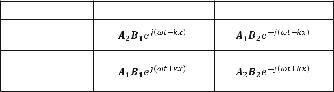
pðx, tÞ ¼ A1B1e jðωtþkxÞ þ A1B2e jðωt kxÞ |
ð |
3:12 |
Þ |
|
þA2B1e jðωt kxÞ þ A2B2e jðωtþkxÞ |
|
||
where A1, A2, B1, and B2 are complex numbers.
The four terms in the above equation can be considered as:
Four Basic Complex Solutions (BCS)
Complex Function |
Complex Conjugate Pair |
Forward Wave
Backward Wave
Because each term of the above equation is a complex solution of the acoustic wave equation and every term is an independent solution, the four basic complex solutions when in complex conjugate pairs can be used to construct any traveling wave.
In addition, every BCS is a complex solution that satisfies the one-dimensional acoustic wave equation Eq.(3.1). This can be proved directly by substituting the BCS into the acoustic wave equation, as shown in Example 2.3 in the previous chapter.
Although the complex solution above p(x, t) is a mathematical solution to the acoustic wave equation, a complex function p(x, t) cannot represent a physical acoustic pressure. For the complex solution p(x, t) to represent an acoustic pressure, it must be a real number resulting from the addition of complex conjugate pairs.
The constant complex coefficients of the four BCSs can be expressed with complex exponentials of explicit phases (CEP) as follows:
A1 =A1e jα1 |
ð3:13Þ |
||
A2 =A2e jα2 |
ð3:14Þ |
||
B1 =B1e jβ1 |
ð3:15Þ |
||
B2 =B2e jβ2 |
ð3:16Þ |
||
where A1, A2 ,B1, and B2 are magnitudes and α1, α2, β1, and β1 are phases. |
|
|
|
Substituting Eq. (3.13) and Eq. (3.16) into Eq.(3.12) yields: |
|
|
|
pðx, tÞ ¼ A1B1e jðωtþkxþα1þβ1Þ þ A1B2e jðωt kx α1 β2Þ |
ð |
3:17 |
Þ |
þA2B1e jðωt kxþα2þβ1Þ þ A2B2e jðωtþkx α2 β2Þ |
|
||
where A1, A2 ,B1, B2, α1, α2, β1, and β1 are real unknown constants that can be determined by the boundary and initial conditions.