
- •Preface
- •Objectives of the Book
- •Style
- •Prerequisites
- •The Big Picture
- •Contents
- •1.1 Review of Complex Numbers
- •1.2 Complex Numbers in Polar Form
- •1.3 Four Equivalent Forms to Represent Harmonic Waves
- •1.4 Mathematical Identity
- •1.5 Derivation of Four Equivalent Forms
- •1.5.1 Obtain Form 2 from Form 1
- •1.5.2 Obtain Form 3 from Form 2
- •1.5.3 Obtain Form 4 from Form 3
- •1.6 Visualization and Numerical Validation of Form 1 and Form 2
- •1.8 Homework Exercises
- •1.9 References of Trigonometric Identities
- •1.9.1 Trigonometric Identities of a Single Angle
- •1.9.2 Trigonometric Identities of Two Angles
- •1.10 A MATLAB Code for Visualization of Form 1 and Form 2
- •2.2 Equation of Continuity
- •2.3 Equation of State
- •2.3.1 Energy Increase due to Work Done
- •2.3.2 Pressure due to Colliding of Gases
- •2.3.3 Derivation of Equation of State
- •2.4 Derivation of Acoustic Wave Equation
- •2.5 Formulas for the Speed of Sound
- •2.5.1 Formula Using Pressure
- •2.5.2 Formula Using Bulk Modulus
- •2.5.3 Formula Using Temperature
- •2.5.4 Formula Using Colliding Speed
- •2.6 Homework Exercises
- •3.1 Review of Partial Differential Equations
- •3.1.1 Complex Solutions of a Partial Differential Equation
- •3.1.2 Trigonometric Solutions of a Partial Differential Equation
- •3.2 Four Basic Complex Solutions
- •3.3 Four Basic Traveling Waves
- •3.4 Four Basic Standing Waves
- •3.5 Conversion Between Traveling and Standing Waves
- •3.6 Wavenumber, Angular Frequency, and Wave Speed
- •3.7 Visualization of Acoustic Waves
- •3.7.1 Plotting Traveling Wave
- •3.7.2 Plotting Standing Wave
- •3.8 Homework Exercises
- •4.2 RMS Pressure
- •4.2.1 RMS Pressure of BTW
- •4.2.2 RMS Pressure of BSW
- •4.3 Acoustic Intensity
- •4.3.1 Acoustic Intensity of BTW
- •4.3.2 Acoustic Intensity of BSW
- •4.5.1 Issues with Real Impedance
- •4.6 Computer Program
- •4.7 Homework Exercises
- •4.8 References
- •4.8.1 Derivatives of Trigonometric and Complex Exponential Functions
- •4.8.2 Trigonometric Integrals
- •5.1 Spherical Coordinate System
- •5.2 Wave Equation in Spherical Coordinate System
- •5.3 Pressure Solutions of Wave Equation in Spherical Coordinate System
- •5.4 Flow Velocity
- •5.4.1 Flow Velocity in Real Format
- •5.4.2 Flow Velocity in Complex Format
- •5.5 RMS Pressure and Acoustic Intensity
- •5.7 Homework Exercises
- •6.1 Review of Pressure and Velocity Formulas for Spherical Waves
- •6.2 Acoustic Waves from a Pulsating Sphere
- •6.3 Acoustic Waves from a Small Pulsating Sphere
- •6.4 Acoustic Waves from a Point Source
- •6.4.1 Point Sources Formulated with Source Strength
- •6.4.2 Flow Rate as Source Strength
- •6.5 Acoustic Intensity and Sound Power
- •6.6 Computer Program
- •6.7 Project
- •6.8 Objective
- •6.9 Homework Exercises
- •7.1 1D Standing Waves Between Two Walls
- •7.2 Natural Frequencies and Mode Shapes in a Pipe
- •7.3 2D Boundary Conditions Between Four Walls
- •7.3.1 2D Standing Wave Solutions of the Wave Equation
- •7.3.2 2D Nature Frequencies Between Four Walls
- •7.3.3 2D Mode Shapes Between Four Walls
- •7.4 3D Boundary Conditions of Rectangular Cavities
- •7.4.1 3D Standing Wave Solutions of the Wave Equation
- •7.4.2 3D Natural Frequencies and Mode Shapes
- •7.5 Homework Exercises
- •8.1 2D Traveling Wave Solutions
- •8.1.2 Wavenumber Vectors in 2D Traveling Wave Solutions
- •8.2 Wavenumber Vectors in Resonant Cavities
- •8.3 Traveling Waves in Resonant Cavities
- •8.4 Wavenumber Vectors in Acoustic Waveguides
- •8.5 Traveling Waves in Acoustic Waveguides
- •8.6 Homework Exercises
- •9.1 Decibel Scale
- •9.1.1 Review of Logarithm Rules
- •9.1.2 Levels and Decibel Scale
- •9.1.3 Decibel Arithmetic
- •9.2 Sound Pressure Levels
- •9.2.2 Sound Power Levels and Decibel Scale
- •9.2.3 Sound Pressure Levels and Decibel Scale
- •9.2.4 Sound Pressure Levels Calculated in Time Domain
- •9.2.5 Sound Pressure Level Calculated in Frequency Domain
- •9.3 Octave Bands
- •9.3.1 Center Frequencies and Upper and Lower Bounds of Octave Bands
- •9.3.2 Lower and Upper Bounds of Octave Band and 1/3 Octave Band
- •9.3.3 Preferred Speech Interference Level (PSIL)
- •9.4 Weighted Sound Pressure Level
- •9.4.1 Logarithm of Weighting
- •9.5 Homework Exercises
- •10.1 Sound Power, Acoustic Intensity, and Energy Density
- •10.2.2 Room Constant
- •10.2.3 Reverberation Time
- •10.3 Room Acoustics
- •10.3.1 Energy Density due to an Acoustic Source
- •10.3.2 Sound Pressure Level due to an Acoustic Source
- •10.4 Transmission Loss due to Acoustical Partitions
- •10.4.2 Transmission Loss (TL)
- •10.5 Noise Reduction due to Acoustical Partitions
- •10.5.1 Energy Density due to a Partition Wall
- •10.5.2 Sound Pressure Level due to a Partition Wall
- •10.5.3 Noise Reduction (NR)
- •10.6 Homework Exercises
- •11.1 Complex Amplitude of Pressure and Acoustic Impedance
- •11.1.3 Transfer Pressure
- •11.2 Complex Acoustic Impedance
- •11.3 Balancing Pressure and Conservation of Mass
- •11.4 Transformation of Pressures
- •11.5 Transformation of Acoustic Impedance
- •11.7 Numerical Method for Molding of Pipelines
- •11.8 Computer Program
- •11.9 Project
- •11.10 Homework Exercises
- •12.1.1 Equivalent Acoustic Impedance of a One-to-Two Pipe
- •12.2 Power Transmission of a One-to-Two Pipe
- •12.3 Low-Pass Filters
- •12.4 High-Pass Filters
- •12.5 Band-Stop Resonator
- •12.6 Numerical Method for Modeling of Pipelines with Side Branches
- •12.7 Project
- •12.8 Homework Exercises
- •Nomenclature
- •Appendices
- •Appendix 1: Discrete Fourier Transform
- •Discrete Fourier Transform
- •Fourier Series for Periodical Time Function
- •Formulas of Discrete Fourier Series
- •Appendix 2: Power Spectral Density
- •Power Spectral Density
- •Accumulated Sound Pressure Square
- •Sound Pressure Level in Each Band
- •References
- •Index

2.2 Equation of Continuity |
|
|
31 |
||||
The governing equation of the cubic can be expressed as: |
|
|
|||||
p þ |
∂p |
|
x y z þ ðpÞ y z ¼ ρ0 x y z ∙ |
∂ |
|||
|
|
∙ |
|
|
v f |
||
∂x |
|
∂t |
|||||
It can be simplified as: |
|
x y z ¼ ρ0 x y z ∙ ∂t v f |
|
|
|||
|
∂x |
∙ |
|
|
|||
|
|
∂p |
∂ |
|
|
When the above equation is compared to Newton’s law of motion, the left-hand
side of the equation is the force ( |
∂p |
∙ |
x |
y z) due to the pressure difference, and the |
|||||
|
|||||||||
|
|
|
∂x |
|
|
|
|
|
|
right-hand side of the equation is the mass (ρ0 |
x y z) multiplied by the accelera- |
||||||||
tion ( |
∂ |
v f ). |
|
|
|
|
|
||
|
|
|
|
|
|
||||
|
∂t |
|
|
|
|
|
|||
Simplifying the equation above |
by |
eliminating |
x y z yields the |
||||||
one-dimensional Euler’s force equation in Cartesian coordinates: |
|||||||||
|
|
|
∂p |
¼ ρ0 |
∂ |
v f |
|
||
|
|
|
|
|
|
||||
|
|
|
∂x |
∂t |
|
The one-dimensional Euler’s force equation above can be extended to threedimensional Euler’s force as:
pðx, y, z, tÞ ¼ ρ0 |
∂ ! |
|||
∂t |
v f ðx, y, z, tÞ |
|||
where both p(x, y, z, t) and |
∂ |
! |
|
|
|
v f ðx, y, z, tÞ are vectors. |
|||
∂t |
2.2Equation of Continuity
The equation of continuity shows the relationship between molecular flow velocity and molecular density. The equation of continuity in Cartesian coordinates is:
∂t |
ρ0 |
ρ0 |
¼ |
∂x þ |
ey |
∂y þ |
ez |
∂z |
∙ !v f |
||
∂ |
ρ |
ex |
∂ |
∂ |
∂ |
||||||
|
|
|
|
b |
|
|
b |
|
b |
|
|
!
where v f is the flow velocity of air molecules; variables x, y, and z are space coordinates; t is time; ρ0 is the averaged molecular density; and ρ is the instantaneous molecular density.
The equation of continuity in vector format is independent of coordinate systems. The equation of continuity in vector format is:

32 |
|
|
|
|
|
|
2 Derivation of Acoustic Wave Equation |
||||||
∂t |
ρ0 |
¼ |
|
|
|
|
|
||||||
|
∂ |
ρ |
ρ0 |
|
|
|
∙ !v f |
|
|
|
|||
The gradient in Cartesian |
|
|
|
|
|
|
|
||||||
coordinates is a vector with bases e , e |
, and e |
: |
|||||||||||
|
|
∂ |
|
∂ |
|
∂ |
bx by |
bz |
|
||||
|
¼ bex |
|
þ bey |
|
|
þ bez |
|
|
|
|
|||
∂x |
∂y |
∂z |
|
|
|
For a one-dimensional plane wave, the equation of continuity in Cartesian
coordinate can be simplified as: |
|
|
¼ ∂x |
|
|
∂t |
ρ0 |
|
|
|
∂ |
ρ |
ρ0 |
∂ v f |
|
|
|
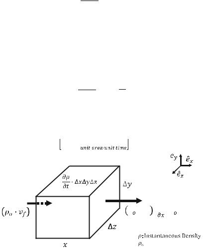
The equation of continuity can be derived from the law of conservation of mass. To simplify the derivation of the equation of continuity, we will use the one-dimensional plane wave in Cartesian coordinate as an example:
Mass flow rate:=
:
Mass passing through an unit area per unit time |
̂ |
+
∆ |
: Average Density |
The above figure illustrates the mass coming in and out of a cubic unit. The mass flow rate,Qρ, is defined as the mass passing through a unit area per unit time. So, the amount of mass passing through a small area, say y z, is equal to Qρ y z t.
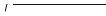
According to the law of conservation of mass, the increase of mass in the cubic unit is equal to the “mass flow in” minus “mass flow out”, as shown in the figure below:

2.2 Equation of Continuity |
33 |
∆ |
∆ ∆ ∆ |
+ |
|
∆ ∆ ∆ ∆ |
|
||||
|
|
|
Increase
Mass in Mass out
of mass
Mass flow rate |
|
||
|
|
|
|
Mass passing through |
: Average Density |
||
an unit area per unit time |
|||
|
The equation of continuity can be concluded as:
∂ρ |
|
|
|
∂Q |
|
|
∙ t ∙ x y z ¼ Qρ ∙ |
y z ∙ |
t Qρ þ |
ρ |
x ∙ y z ∙ t |
∂t |
∂x |
We will compare the above equation to the law of conservation of mass.
The left-hand side of the equation is the increase of mass in this cubic unit
( |
∂ρ |
∙ t ∙ x y z) after a finite time ( |
t). |
|
|
|
|
||||||
|
|
|
|
|
|||||||||
|
∂t |
|
|
|
|
|
|
y z ∙ t) minus the |
|||||
|
|
The right-hand side of the equation is the mass flow in (Qρ ∙ |
|||||||||||
mass flow out ( Qρ þ |
∂Qρ |
|
x ∙ y z ∙ |
t). The above equation can be simplified to: |
|||||||||
∂x |
|||||||||||||
|
|
|
∂ρ |
|
|
|
∂Q |
|
|||||
|
|
|
|
∙ t ∙ |
x y z ¼ |
ρ |
|
x ∙ y z ∙ |
t |
||||
|
|
|
∂t |
∂x |
|||||||||
and: |
|
|
|
|
|
|
|
||||||
|
|
|
|
|
|
|
∂ρ |
¼ |
∂Qρ |
|
|||
|
|
|
|
|
|
|
|
|
|
|
|||
|
|
|
|
|
|
|
∂t |
∂x |
|
||||
|
|
The mass flow Qρ is replaced with ρovf to get: |
|
||||||||||
|
|
|
|
|
|
|
∂t ¼ ∂x ρov f |
|
|||||
|
|
|
|
|
|
|
∂ρ |
|
∂ |
|
|
|
|
This is the one-dimensional equation of continuity in Cartesian coordinates.