

80 |
8 Application of Chaos Theory to Acoustical Imaging |
Fig. 8.10 Image obtained by born approximation. After Jia and Han [14]
The root mean square values of the pixels of the images formed by Born approximation and fractal approximation are given by Eqs. (8.30), (8.31). The fractal approximation shows a smaller value with respect to the original image. This shows that the fractal approximation is a better technique. Generally, Figs. 8.11, and 8.12 show images obtained by fractal approximation of Hankel function.
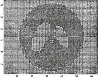
K0 is chosen as 1 or 2 in the Bessel function of Third Order-Hankel function [21]. If K0 is changed to 300, Fig. 8.11 shows that the image obtained is distorted. The main ellipses within the phantom have been ignored during the calculation of the Bessel function. A value of 1 or 2 is suggested for K0 because Fig. 8.12 is the mesh plot of Fig. 8.11.
8.18Comparison Between Born and Fractal Approximation
In general, images from Born approximation and fractal approximation both suffer from severe artefacts. There are reasons for this. One is the number of iterations is insigniÞcant in bringing the initial guess of the object function closer to the Þnal result. The second reason is due to the image resolution is based only on 64 × 64 projection samples. This is considered very low in resolution for medical or image processing standard. Thus artefacts can be reduced with more rounds of iterations and higher resolution [3]. The differences between Born approximation and fractal approximation are still noticeable in the images although the limited rounds are
8.18 Comparison Between Born and Fractal Approximation |
81 |
Fig. 8.11 Image obtained by fractal approximation of Hankel function K0 = 300, P colour Plot. From Jia and Han [14]
Fig. 8.12 Image obtained by fractal approximation of Hankel Function K0 = 300, Mesh Plot. From Jia and Han [14]
82 |
8 Application of Chaos Theory to Acoustical Imaging |
iterations are not able to bring out the progressive convergence of the Kaczmarz algorithm. An obvious difference is shown in the presence of the boundary of the main ellipse in the images based on the fractal approximation. Also the boundary of the object is established at such an early stage of iteration of the fractal approximation. This marks a clear improvement over the Born approximation. The reduction of the magnitude of the artefacts is within the object is another improvement. This is shown by the intensity of the colour within the objectÕs boundary reduces whereas the colour intensity of images remains unchanged when based on the Born approximation [3].
References
1.Gan, Woon Siong. 1992. Application of chaos to sound propagation in random media. In Acoustical Imaging, vol. 19,99Ð102,ed. H. Ermert, and H. Harjes. New York: Plenum Press.
2.http://library.thinkquest.org/3120/test/c-his1.htm.
3.Chow, W.H. 2002. Acoustic Fractal Imaging Using Diffraction Tomography. M.Eng. thesis, Nanyang Technological University, chapter 5, p. 112.
4.Gleick, J. 1981. Chaos-Making A New Science, 29. New York: McGraw Hill.
5.Laplante, P., Fractal Mania, Windcrest/McGraw Hill, USA.
6.Gan, W.S., and C.K. Gan. 1993. Acoustical Fractal Images Applied to Medical Imaging, Acoustical Imaging, vol.20, 413Ð416. Plenum Press, New York.
7.Lam, C.K., and E.H. Lau. 1996. Acoustical Chaotic Image for Medical Imaging. B.Eng. Thesis, NTU.
8.Kjems, J.K. 1996. Fractals and experiments. In Fractals and Disordered System, 2nd ed., 284Ð286. Berlin: Springer.
9.Stanley, H.E. 1996. Fractals and multifractals: the interplay of physics and chemistry. In Fractals and Disordered Systems, 2nd ed., 1Ð13. Berlin: Springer.
10.http://members.home.net/jason.jiin/content/.htm.
11.Leeman, S., E.T. Costa. 1993. Large aperture hydrophones for far Þeld measurement and calibration, IEE, London. Acoustic Sensing & Imaging, 294.
12.Sander, L.M. 1987. Fractal Growth, 94. ScientiÞc American.
13.Vicsek, T. 1989. Fractal Growth Phenomena,1st ed, 158Ð167. Singapore: World ScientiÞc.
14.Jia, Yu, and Chan Tuck Han. 2003. Development of an Ultrasound Imaging Algorithm for Detecting Breast Cancer. B.Eng. Thesis, NTU.
15.Bunde, A., and S. Havlin (eds.). 1996. Fractals and Distorted Systems, 2nd ed., 7. Berlin: Springer.
16.Kaveh, M., M. Soumekh, and R.K. Mueller. 1986. A comparison of Born and Rylov approximatin in acoustic tomography. Acoustical Imaging 14: 325Ð334.
17.http://www.nr.com/Numerical Recipes in Chapter 2.
18.Kaczmarz, S. 1937. Angena¨ herte Außo¨ sung von Systemen Linearer Gleichungen. Bulletin Academie Polonaise Sciences et Lettres A 355Ð357.
19.Ramakrishnan, R.S., S.K.J. Mullick, R.K.S. Rathore, and R. Subramanian. 1979. Orthogonalisation, Bernstein polynomials and image restoration. Applied Optics 18: 464Ð468.
20.HounsÞeld, G.N. A method of apparatus for examination of a body by radiation such as x ray or gamma radiation. Patent SpeciÞcation, The Patent OfÞce.
21.Slaney, M., and A.C. Kak. 1985. Imaging with Diffraction Tomography, 39. University of Purdue Internal Report, TR-EE 85-5.

Chapter 9
Nonclassical Nonlinear Acoustical
Imaging
9.1 Introduction
A traditional view of classical nonlinearity of nonlinear ultrasonics is based on the idea of elastic waveform distortion due to material nonlinearity. This waveform distortion is due to the variation in local sound velocity as the sound wave propagates in the material. This sound velocity variation is accumulated with propagation distance resulting in the progressive transition of the incident harmonic wave into the sawtooth or N-type wave. The consequence is that the spectrum acquires higher harmonics of the fundamental frequency which provide information on the material. For sound propagation in free-from-defects media, the material nonlinearity is rather low and a few harmonics are observable. Hence classical nonlinear nondestructive testing (NDT) is basically second harmonic NDT.
Nonclassical nonlinear acoustical imaging involves nonclassical contact acoustic nonlinearity (CAN) [1] spectra. Nonclassical nonlinear acoustical imaging has applications in material characterization and nondestructive testing. In these two applications, two forms of nonclassical acoustic nonlinearity are involved with, the mesoscopic or hysteretic nonlinearity and contact acoustic nonlinearity (CAN). Mesoscopic nonlinearity originates from the bond system of inclusions like dislocations, cracks, grain contacts etc. and in heterogeneous materials. This results in a hysteretic stress–strain and strongly nonlinear relation. The nondestructive testing applications are related to the study of the slow dynamic behaviour of the hysteretic materials. This is a strong mechanical impact followed by a slow recovery. The latter is an indication of the presence of defects. It is robust methodology for a pass/nonpass evaluation in nondestructive testing.
The contact acoustic nonlinearity (CAN) is caused by the mechanical constraint between the fragments of planar defects which make their vibrations extremely nonlinear. CAN in general manifests in a wide class of damaged materials. Multiple ultraharmonics are efficiently generated by the cracked defects which also support multiwave interactions. The planar defects also have resonance properties bringing in
© Springer Nature Singapore Pte Ltd. 2021 |
83 |
W. S. Gan, Nonlinear Acoustical Imaging, https://doi.org/10.1007/978-981-16-7015-2_9