for all odd integers of k and nonzero for all even integers of k. For example

8.6.3 Other Definitions

From the comparison of Eqs. (8.5) with (8.6), one Þnds that the displacement of the random walking and can be deÞned as

This shows that the characteristic length L 2 and L4 have the same asymptotic dependence on time. The leading exponent in the above equation is known as the scaling exponent and the nonleading exponent known as the corrections-to-scaling exponent. Extending to any length L k , provided k is even, a general equation can be obtained as follows:

The subscripts on the amplitudes indicate their k-dependence. The above equation displays the robust feature of random system. Also despite different deÞnitions of characteristic length, the asymptotic behaviour is described by the same scaling exponent.

8.7 Fractal Approximations

Scientists at the Mount Sinai School of Medicine in New York City have successfully demonstrated that the fractal structure inside cells can indicate breast cancer [3]. Besides this, other works [6Ð8] have conÞrmed the chaotic nature of the scattering of ultrasound. Hence a fractal growth model can be used to adequately describe the scattered Þeld within the breast.

From this, a new approximation method-the Fractal Approximation (FA) has been proposed by Leeman and Costa [11] based on the assumption that the scattered Þeld

The fractal growth probability distribution function P(r, t) is introduced for the modiÞcation. The distribution function in turn is based on the fractal growth model known as the Diffusion Limited Aggregation (DLA) [12].

8.8 Diffusion Limited Aggregation

It has been discovered by scientists that many diverse natural phenomena have similar fractal shapes. That is, they are self-similar under different scaling factors. For instance, percolation clusters, a form of fractals are used to describe patterns created by water as it ßows through coffee grinds or seeps into the soil. Comparable fractal patterns are also generated by the growth of some crystals and electrical charges.

Sander [12] and Thomas A. Witten in 1987 developed a model for fractal growth known as Diffusion Limited Aggregation (DLA). A random and irreversible growth process is used to create a particular type of fractal for their model. Today DLA has about 50 realizations in physical systems and much of current interest on fractals in nature are focused on FLA [12].

Aggregation is the process of growth of many clusters in nature. This means one particle after another comes into contact with a cluster and remains Þxed in place. The resulting process is DLA if these particles diffuse toward the growing cluster along random walks [13].

Their research has the main assumption that the scattering paths of ultrasound in

the breast follow the fractal-like structure of the DLAs. Therefore, one can model

−→

the internal scattered Þeld us ( r ) with the fractal growth model.

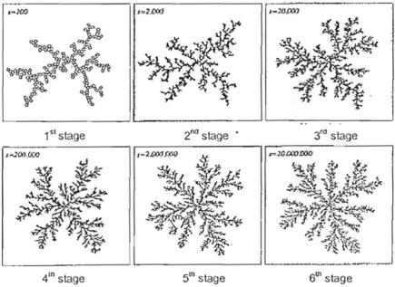
To generate and grow a DLA cluster, Þrst a seed particle is placed at the origin. This is followed by the release of random walkers one at a time, from some distant locations around the circumference of a circle surrounding the site of the origin.

When one of these particles makes contact with the seed at the origin, it sticks and forms an aggregate followed by the release of the next particle. The particle will be considered void and removed if it touches the boundary of the circle before reaching the origin. Self-similar clusters shown in Fig. 8.6 will be created by the totally random motion of the particles. It is noted that the dimension of the clusters increases as represented by s.

8.9 Growth Site Probability Distribution

From the description in previous section, it shows that DLA cluster is a form of probability. Here each step of a random walker is governed and described by a probability distribution known as the Growth Site Probability Distribution (GSPD) [15].

Fig. 8.6 A two dimension DLA clusters at six different stages of growth. After Sander [12]

There are a few types of GSPD in existence. In this chapter, one will consider the diffusion process of a random walker who is slowed down by entanglements such as dangling ends, large holes and bottlenecks [15]. This type is chosen because the scattering of ultrasound is also affected by the internal structure of the object which is inhomogeneous and the surrounding medium.

Averaging this distribution over all the starting points of the random walkers, which are the coordinates of each sample point in the projection of the forwardscattered Þeld, the probability distribution reduces to a stretched version of the Gaussian distribution [15]. Then the distribution P (r, t ) is given by the following expression:

where P (0, t ) = the average probability of Þnding a random walker at the starting point, r 2(t ) 1/2 = the root mean square distance of the walker from the starting point, and dw = fractal dimension of a random walk or the diffusion exponent.

There is a strong evidence that Eq. (8.11) is valid for a large class of random fractals [6Ð8]. From the above equation, the average GSPD, P (r, t ) is given by:

where η = dw .

dw −1

With a long time span, the average probability at the starting point, P (0, t ) is proportional to the inverse of the number of distinctly visited sites, S(t).S(t) scales as r 2(t ) d f /2 on fractals, and one has

where d f = fractal dimension of the DLA cluster, and dw = the diffusion exponent. It is mentioned earlier that the motion of the random walker is assumed to be slowed down by entanglements. Hence the root mean square distance of the walker

is given by a more general power law [6Ð8] as:

With the substitution of (8.14), (8.13) into (8.12), the GSPD is then given by

This shows that there are two unknown parameters which have to be deÞned: dw , the diffusion coefÞcient and d f , the fractal dimension of the DLA cluster.

8.10 Approximating of the Scattered Field Using GSPD

With the general equation of GSPD, it can be applied to the modelling of the ultrasound scattered Þeld within the breast. In diffraction tomography, the general expression for the incident Þeld, assuming plane wave, is given by

k2, r = (x , y)T and k = wave number.

Multiplying the incident wave Þeld with the GSPD, the scattered ultrasound Þeld within the object is