

Chapter 8
Application of Chaos Theory to Acoustical Imaging
8.1Nonlinear Problem Encountered in Diffraction Tomography
Woon Siong Gan [1] is the Þrst to introduce the concept of chaos theory to acoustical imaging in 1990. It was applied to the nonlinear problems encountered to obtain the expression for the scattered Þeld in the imaging modality of diffraction tomography. Diffraction tomography is a common method used in medical ultrasound imaging such as for breast imaging. Breast tissue being inhomogeneous will cause, multiple scatterings on the sound wave propagating in the medium. This is a breakthrough in diffraction tomography as the usual approach is Born and Rytov approximations in the solving the nonlinear problem of the LippmanÐSchwinger integral in diffraction tomography. These are linear and Þrst order approximations.
Based on the mathematical theorem that every nonlinear differential equation has a chaos solution subjected to certain conditions. Since the LippmanÐSchwinger integral is a nonlinear differential equation, it will have chaos solutions. Chaos phenomena have fractal characteristics geometrically. That is the chaos solution will give to fractal images. Since there is a key property of chaos that it is very sensitive to the initial condition, the fractal images produced should be able to show very Þne changes in the condition of the object. For the case of breast imaging it will be useful for the detection of early stage cancer.
A background on chaos theory and fractal images will be given followed by the implementation in the solution of the LippmannÐSchwinger integral and then the formation of the fractal images. Then the application to medical ultrasound imaging will be given with an illustration by breast imaging.
© Springer Nature Singapore Pte Ltd. 2021 |
61 |
W. S. Gan, Nonlinear Acoustical Imaging, https://doi.org/10.1007/978-981-16-7015-2_8
62 |
8 Application of Chaos Theory to Acoustical Imaging |
8.2 Definition and History of Chaos
The usual meaning of the word ÔchaosÕ is a state of disorder or confusion and is equivalent to randomness. This can be applied to most cases but is not applicable when one considers the mathematical theory of chaos. The mathematical theory of chaos was discovered in the 1960s by Edward Lorenz, a meteorologist. He was attempting to predict the weather through the use of a mathematical model. He managed to generate a theoretical sequence of weather predictions using computer [2].
In a different attempt to observe the sequence of weather pattern, in order to save time, he ran the problem from the middle of the sequence. He was surprised to Þnd that the results deviated from the previous sequence. He found that the error was due to a slight truncation in the decimal places of the values used. With this discovery, Lorenz began to establish the mathematical theory of chaos by relating this to the effect of a butterßy in the prediction of weather [2]. The ßapping of a single butterßyÕs wing today produces a tiny change in the state of the atmosphere. Over a period of time, the atmosphere diverges from what it would have done. Therefore in one month time, a tornado that would have devastated the Indonesian coast does not happen. Or, perhaps the event that was not going to happen, happens [3]. These phenomena are known in chaos theory to be the sensitive dependence on initial condition.
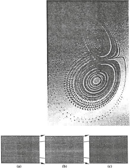
Lorenz concluded that it is impossible to predict the weather since slight factor can affect it so drastically. He thereby proceeded to simplify his model for weather forecast and developed a set of three simple equations that have a sensitive dependence on initial conditions. These equations would generate a sequence of random behaviour. He was surprised to note that an inÞnite, double spiral known as the Lorenz Attractor was generated when the equations were plotted (Fig. 8.1).
The output ßuctuated within the spirals. Gleick [4] discovered that these equations described the water wheel system exactly.
8.3 Definition of Fractal
The word ÔfractalÕ was coined by Benoit Mandelbrot from the Latin adjective fractus. It has the meaning of being fragmented and irregular. It was created to describe a rough geometric Þgure that has the property of self-similarity or its statistical average. Self-similarity of a single item means that the item has a repetitive nature of itself when it is viewed under different length scales. This is shown in Fig. 8.2 which shows a Mandelbrot set, a computer-generated fractal. Figure 8.2a shows the Mandelbrot set at a particular viewing angle. By zooming in on this Þgure, a similar Þgure of the Mandelbrot set is obtained as shown in Fig. 8.2b (deÞned by the grey box). A further zooming reconÞrms the repetitive nature of the fractal as shown in Fig. 8.2c.
8.4 The Link Between Chaos and Fractals |
63 |
Fig. 8.1 3-D Lorentz Attractor. From http://astron omy.swin.edu.au/pbourke/fra ctals/lorenz/
Fig. 8.2 Zooming in of Mandelbrot set (from left to right). From Hsiang (2002)
8.4 The Link Between Chaos and Fractals
The above is a general introduction to chaos and fractals. Next one will describe the link between them. From careful observation, one will notice that fractals are actually the visible representations of chaotic systems. If one examines the Lorenz
64
Table 8.1 Different classiÞcation of cellular automata [5]
|
8 Application of Chaos Theory to Acoustical Imaging |
|
|
|
|
Class 1 |
|
Evolution to a homogeneous state (an attractor) |
|
|
|
Class 2 |
|
Evolution to isolated periodic segments |
|
|
|
Class 3 |
|
Evolution that is always chaotic |
|
|
|
Class 4 |
|
Evolution to isolated chaotic segments |
|
|
|
attractor (Fig. 8.1) carefully one will notice that the Þgure is actually a fractal, since it is a visible representation of the chaotic system of the water wheel. An alternative way to study the link between chaos and fractals is to study cellular automata. This is a form of mathematical abstraction from a dynamical system. This has been used for the modelling of massively parallel computer and biological cell behaviour [5].
Cellular automata consists of a space of unit cells and these are initialized by Ô1Õ for living cell and Ô0Õ for unoccupied or dead cell. Besides this, the evolution of these cells is governed by a rule which bases the contents of the cell at time t by its contents at time t Ð 1. With this rule, different cellular automata can evolve which eventually end up with stable, fractal-like formation. With this classiÞcation rule for the cellular automata, a relationship given in Table 8.1 can be established with chaos [5].
8.5 The Fractal Nature of Breast Cancer
The fractal patterns inside cells can reveal breast cancer as this have been successfully shown by scientists at Mount Sinai School of Medicine (Fig. 8.3).
Traditionally pathologists must detect breast cancer by studying individual cells from suspicious tissues and checking for abnormal-looking cell shapes and features through subjective means. The Mount Sinai researchers have studied the distribution of chromatin and DNAÐprotein compounds which contain the chromosomes in a cell by looking within the cell nucleus using the analysis of images of actual breast cells. Like many other biological structures in nature, chromatin forms fractal patterns meaning that the chromatin has similar arrangement over a range of size scales. They apply techniques to study cells from 41 patients of whom 22 were known to have breast cancer from independent means. In a blind study, they correctly diagnosed 39 out of 41 cases, that is with a success rate of 95.1%. This was done by measuring the differences in lacunarity and differences in fractal dimensions between malignant and benign cells. Lucunarity is the size of gaps between chromatin regions in the nucleus and fractal dimension describes how fully a fractal object Þlls up the space is occupied.
There are other works [6Ð8] that conÞrmed the scattering of ultrasound to be chaotic in nature. With these works, one can conÞdently conclude that the fractal growth model can be used to represent the scattered Þeld within the breast due to the fact that all chaotic systems can be represented by fractals.