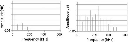
Fig. 7.4 Higher harmonics results of an undamaged circuit board ceramics on the left, and a damaged one on the right. (After Haller [4])

as a receiver. In the recorded frequency spectrum, higher harmonics are detected to indicate the amount of cracks or defects.

The sample used for the experiment is the ceramic semiconductor mounted to the printed circuit board. Higher harmonics was present.

When the semiconductor was damaged. This indicates that either the board itself gives nonlinear response or some component mounted was damaged. After testing a larger number of boards indicated that the nonlinear response arose from the board. When the semiconductors were damaged, the number of multiple harmonics increased and also the amplitude of the harmonics increased. This was shown in Fig. 7.4.

The method of harmonic imaging is convenient for circuit boards with no impacts is present because one has to be careful with the Semiconductor component.

7.8Application of Ultrasound Harmonic Imaging to Underwater Acoustics

Ultrasound harmonic imaging can be applied in active sonar [12]. Prieur et al. [12] developed an active sonar that can receive at both the fundamental and second harmonic frequencies as an aid for target classification. They confirmed the presence of harmonic signals by measuring the pressure field radiated by the circular transducers with a centre frequency of 120 KHz for the first one and 200 KHz for the second one in a water tank up to 12 m range. These measurements also gave them the opportunity to compare with their numerical simulations. They then showed that second harmonic imaging could be used for target detection by imaging spherical targets using a pulse-echo technique. This showed better resolution capabilities compared to images obtained with the fundamental signal. They then used numerical simulations of the pressure field and the active sonar equation to estimate the maximum useful range of the fundamental signal. They also suggested the advantages of combining second harmonic signal with the fundamental signal.

After the confirmation experimentally from the measured profiles that higher harmonics were present and detectable, they set up an experiment for the second.

Experiment for the second harmonic pulse-echo imaging. They set up an experiment using a ES120-7C transducer with a centre frequency of 121 KHz to send a pulse that reflected on targets with the second harmonic at 242 KHz recorded by the ES200-7C transducer.

Both transducers were set side by side. The targets were four spheres. These spheres were made of tungsten carbide and the fourth sphere made of copper. They were all positioned on the horizontal plane which contained the propagation axis of both transducers. The transducer ES200-7C was connected directly to the oscilloscope. The transducers were rotated counter clockwise to cover an angular range of approximately 1.5–4.5°. 0° is the direction parallel to the wall of the water tank and the positive angle is taken in the clockwise direction. The recorded data were processed to filter out the pulse around the fundamental and the second harmonic bands.

The echoes from the three biggest spheres were clearly visible. The echo from the smallest sphere is barely noticeable when filtering around the fundamental frequency while filtering around the second harmonic it is clear. This is caused by the wider main lobe of the fundamental signal compared to the main lobe of the second harmonic signal.

The experiment shows that it is possible to use the second harmonic signal for imaging spheres. The image obtained by using the signal around the second harmonic frequency shows better resolving capabilities and reveals one target that fundamental imaging does not detect. The second harmonic signal has a larger main-lobe-to-side- lobe ratio and this is beneficial for target imaging. In a shallow-water environment, surface and bottom refractions of the side-lobes will cause perturbation to the sonar scanning at low grazing angles. There will also be perturbations from scatters situated in the propagation direction of the side lobes. Due to the lower side-lobe levels, the amplitude of these perturbations will be reduced in second harmonic imaging.

The combination of echoes around the fundamental and second harmonic frequency bands has the advantage that it gives an update that is twice the rate of a sonar receiving echoes around the fundamental frequency only. With the two images obtained, one can combine the high resolution of the second harmonic signal at short range and the long-range capability of the fundamental with a lower resolution.

The second harmonic signal exhibits low side-lobes relative to the main lobe. This is useful in many applications of sonar imaging. Combining echoes from the fundamental and second harmonic signals doubles the data rate per ping. In addition, the echoes at two different frequencies can contribute to target classification, for instance, living organisms, by comparing their frequency response. This is an application of the second harmonic signal in fisheries research.

High transmitted power is needed in this work on the application of second harmonic imaging to active sonar. With low input power the higher harmonics signals generated due to nonlinear propagation are negligible. Medium-to-high input powers are necessary. In the experiment of Prieur et al. [12], 1 kW input power was sufficient to achieve second harmonic imaging. By increasing input power there are

limitations caused by cavitation, hard shock or saturation that all dissipate energy into the medium. Besides this, the receiver has to be sensitive enough to detect the low level of the echoes and the uncertainty of the recorded level has to be small for use in organism characterization.

References

1.Beyer, R.T. 1997. Nonlinear acoustics. Acoustical Society of America.

2.Earnshaw, S. 1860. On the mathematical theory of sound. Philosophical Transactions of the Royal Society of London 150: 133–148.

3.Enflo, B.D., and Hedberg, C.M. 2002. Theory of nonlinear acoustics in fluids. Kluwer Academic Publishers.

4.Haller, K. 2007. Nonlinear acoustics applied to nondestructive testing, Ph.D. thesis, Sweden: published by Blekinge Institute of Technology.

5.Hedrick, W.R., Hykes, D.L., Starchman, D.E. 2005. Ultrasound Physics and Instrumentation. 14th edition. MV, Mosby: St. Louis.

6.Lencioni, R., D. Cioni, and C. Bartolozzi. 2002. Tissue harmonic and contrast-specific imaging: back to gray scale in ultrasound. European Radiology 12: 151–165.

7.Tranquart, F., N. Grenier, V. Eder, and L. Pourcelot. 1999. Clinical use of ultrasound tissue harmonic imaging. Ultrasound in Medicine and Biology 25: 889–894.

8.Buck, O., W.L. Morris, and J.M. Richjardson. 1978. Acoustic harmonic generation at unbonded interfaces and fatigue cracks. Applied Physics Letters 35 (5): 31–373.

9.Barnard, D.J., G.E. Dace, D.K. Rehbein, and O. Buck. 1997. Acoustic harmonic generation at diffusion bond. Journal of Nondestructive Evaluation 16 (2): 77–89.

10.Averkiou, M.A., M.A. Roundhill, and D.R. Powers. 1997. A new imaging technique based on the nonlinear properties of tissues. Proceeding IEEE Ultrasonic Symposium 2: 1561–1566.

11.Hedrick, W.R., and L. Metzger. 2005. Tissue harmonic imaging, a review. Journal of Diagnostic Medical Sonography 21 (3): 183–189.

12.Prieur, F., Nasholm, S.P., Austeng, A., Tichy, F., and Holm, S. 2012. Feasibility of second harmonic imaging in active sonar: measurements and simulation. IEEE Journal of Ocean Engineering 37(3): 3467–3477.