


Chapter 6
B/A Nonlinear Parameter Acoustical
Imaging
6.1 Introduction
The B/A nonlinearity parameter measures the nonlinearity of the equation of state for a fluid. It determines the distortion of a finite amplitude wave propagating in the fluid and the nonlinear correction to the velocity due to the nonlinear effects from the propagation of the finite amplitude wave. Besides this, it is also related to the molecular dynamics of the medium. Thus it can provide informations on the structural properties of the medium such as inter-molecular spacing, clustering, internal pressures, and the acoustic properties of the materials. Hence it is an important physical constant of characterizing the different acoustic materials and biological media [1, 2].
B/A nonlinear parameter is very useful in the medical applications of ultrasound, both in therapeutics and in diagnostics. In medical therapeutics, it enables the prediction of the temperature in the tissue during the ultrasonic hyperthermia treatment. In the diagnostics applications, B/A information can be used in the design and optimization of the ultrasound imaging devices.
There are two basic approaches in the experimental measurement of the B/A nonlinearity parameter: the thermodynamic method and the finite amplitude method.
6.2 The Thermodynamic Method
6.2.1 Theory
The equation of state p = p(ρ, s) of a liquid, in thermodynamics can be expanded into a Taylor series along the isentrope s = s0, as [3]
p − p0 = A ρ + |
2 |
|
ρ |
|
2 |
+ |
3 |
|
ρ |
(6.1) |
||||||
|
ρ |
|
B |
|
ρ |
|
|
|
|
C |
|
ρ |
|
|
||
0 |
|
|
! |
0 |
|
|
|
|
|
! |
0 |
|
|
|||
© Springer Nature Singapore Pte Ltd. 2021 |
37 |
W. S. Gan, Nonlinear Acoustical Imaging, https://doi.org/10.1007/978-981-16-7015-2_6
38 |
6 B/A Nonlinear Parameter Acoustical Imaging |
where ρ’ = ρ − ρ0 = excess density, p = instantaneous pressure, ρ = instantaneous density of the liquid disturbed by the ultrasonic wave propagation, p0, ρ0 = their unperturbed (ambient) values and
A = ρ0 |
|
∂ p |
|
|
|
|
|
= ρ0c02 |
(6.2) |
|||
|
∂ρ |
s |
|
|
||||||||
|
|
|
|
|
|
|
|
|
ρ=ρ0 |
|
||
|
|
|
|
|
|
|
∂ 2 p |
|
|
|||
B = |
ρ02 |
|
|
|
|
s |
(6.3) |
|||||
∂ρ2 |
|
|||||||||||
|
|
|
|
|
|
|
|
|
|
|
ρ=ρ0 |
|
|
|
|
|
|
|
∂ 3 |
|
|
|
|
||
C = |
ρ03 |
|
p s |
(6.4) |
||||||||
∂ρ3 |
||||||||||||
|
|
|
|
|
|
|
|
|
|
|
ρ=ρ0 |
|
where s = specific entropy, c0 = isentropic small signal sound speed. Subscript s denotes constant entropy process which is a condition for the ultrasound propagation. Also the partial derivatives are evaluated at the unperturbed state of (ρ0, s0).
From (6.2) and (6.3), B/A the nonlinearity parameter which is the ratio of the quadratic to the linear term in the Taylor series can be expressed as:
|
|
B |
|
ρ0 |
∂ 2 p |
|
|
|
|
||
|
|
|
= |
|
|
|
|
|
|
|
(6.5) |
|
|
A |
c2 |
∂ρ2 |
|
|
|||||
|
|
|
0 |
|
|
|
s |
ρ=ρ0 |
|
||
|
|
|
|
|
|
|
|
|
|
||
With the definition of sound speed c2 = |
∂ p |
|
|
|
|||||||
∂ρ s |
, (6.5) can be written as |
|
|||||||||
|
A = 2ρ0c0 |
∂ p s |
(6.6) |
||||||||
|
B |
|
|
|
|
∂ c |
|
|
|
||
ρ=ρ0
The partial derivative |
|
∂ c |
|
|
can be further expanded [3] giving |
|
||||||||
|
∂ p |
s |
|
|
||||||||||
|
|
|
|
|
ρ=ρ0 |
|
|
|
|
|
|
|||
|
|
|
|
|
|
|
|
|
|
|
|
|||
|
|
|
|
|
|
|
|
|
|
|
|
|
||
|
B |
= |
2ρ0c0 |
|
∂ c |
T |
+ |
(2 c0 Tq/c0c p ) |
|
∂ c |
p |
|
(6.7) |
|
|
A |
∂ p |
∂ T |
|||||||||||
|
|
|
ρ=ρ0 |
|
||||||||||
|
|
|
|
|
|
|
|
ρ=ρ0 |
|
|
|
|
|
|
where ρ0 = density of undisturbed medium, c0 = sound velocity for acoustic waves of infinitesimal amplitude, c = measured sound velocity at given temperature and pressure, p = acoustic pressure, T = absolute temperature in Kelvin, c p = specific
heat1at |
constant pressure, and q |
= |
isobaric volume coefficient of thermal expansion |
|||
∂ V |
|
|
||||
= ( |
|
) |
∂ T |
p . |
|
|
V |
|
|
||||
6.2 The Thermodynamic Method |
39 |
6.2.2 Experiment
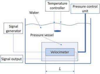
Equation (6.7) indicates that it is necessary to measure the sound velocity as a function of pressure and temperature accurately in the investigated medium in order to determine B/A. To use the thermodynamic method, a velocimeter is required. This is a vessel of known length L, comprising the test liquid and the transmitter–receiver equipment inserted in a liquid-filled pressure vessel such as water or oil that is in turn submerged in a bath with controlled temperature (Fig. 6.1).
The first term of Eq. (6.7) is known as the isothermal nonlinear parameter and the second term is referred to as the isobaric nonlinear parameter. This second term of Eq. (6.7) is used for the thermodynamic method for determination of B/A. The speed of sound measurement can be performed with different techniques to infer the travel time (time of flight), ttr of the sound wave through the velocimeter of known length L. (Fig. 6.1). The first paper on the determination of B/A using the thermodynamic method is that of Beyer [3]. Greenspan and Tschiegg [5] used a sing-around circuit to infer ttr , ttr is inferred through the pulse repetition frequency (PRF) as the circuit allows for the triggering of the generator to send a pulse once the preceding pulse is received. The accuracy of the measurement was improved by Greenspan et al. [6] by adjusting the PRF of the generator for a new pulse to be transmitted when the echoes of the previously transmitted pulse were superimposed on the receiver.
In this way, the device can measure the speed of sound from the pulse transit time ttr , inferred from the distance travelled by the pulse equal to twice the the length of the vessel and the PRF:
Fig. 6.1 Schematic simplified diagram of the typical setup used for a thermodynamic B/A measurement (After Panfilova [4])