Катин МОЛЕЦУЛАР ДЫНАМИЦС ИН МУЛТИСЦАЛЕ МОДЕЛИНГ 2015

3

4

Preface

In the frame of the course students learn the basic theoretical fundament of the molecular dynamics (MD) simulations. We pay attention to physical and mathematical ideas of MD simulations rather than the interface of corresponding software. Students create their own programs for simple MD calculations and the special packages they use only in the second part of the semester. So, the initial skills in programming are implemented. Three examples of the multiscale modeling that demonstrate different aspects of the using of MD methods are included in this textbook.

The course contains 37 exercises of different complexity from simple to laborious. Depending on the level of training group, these exercises can be discussed during the lectures or can be given as the homework. High-motivated students may read original articles and make presentations on the subject.

The course is addressed to students, specialized in condensed matter physics, chemical physics and quantum chemistry.

Introduction

Molecular dynamics (MD) is the complex of algorithms for computer modeling of the atoms and molecules motion in a “real-time mode”.

MD is a powerful tool for the matter modeling in the atomic scale. It is useful for nanoclusters, solids and liquids studying. Chemical reactions, thermal stability, phase transitions, adsorption/desorption and many other processes can be investigated using MD.

The main challenge of MD methods is caused by insufficient computer performance, which allows to study of a limited number of atoms (usually from a few tens to a few tens of thousands) for a relative short period (usually in a picoseconds scale, seldom up to a few microseconds). If the larger systems or the longer times are needed, then the different extrapolation techniques should be applied to transfer results obtained for the small systems to the large objects. One of such technique is the multiscale modeling. In this approach, consistent simulations on the different scales are implemented. In the frame of multiscale modeling, MD usually plays a role of the lowest (basic) level and provides data required for the higher-level simulation.

5

System of units

In MD simulations one deals with atomic scaled quantities, thus the International System of Units (SI) is not suitable. Here we propose another system based on three basic units: angstrom (1 Å = 10-10 meters), femtosecond (1 fs = 10-15 seconds) and electron-volt (1 eV = = 1.6·10-19 Joules). The other units should be derived from the basic units. For example, velocities should be measured in Å/fs, forces should be measured in eV/Å, masses should be measured in eV (fs/Å)2, etc. The system of units proposed is a natural system for the molecules. Therefore, it provides the possibility to avoid too large and too small quantities in MD simulations.

Exercise 1. Please find the values of the followed physical quantities expressed using the molecular system of units: mass of the water molecule, mean velocity of the nitrogen molecule at room temperature (300 K), 500 GHz oscillation frequency, 2 nN force.

Common approximations

The atomic motion is defined by both atomic nuclei and electrons properties. Despite of electrons have a negligible mass, they play a crucial role in the interatomic interactions. The common approximation is to represent nuclei as classical particles moving along the classical trajectories. Interaction forces are partially associated with electronic subsystem, which can be accounted for at classical or quantum level of theory. This simplified assumption is not always correct for light nuclei (especially for hydrogen nucleus), which can exhibit quantum properties (for instance, quantum tunneling). Nevertheless, it is acceptable in most cases. The other common assumption is so-called adiabatic approximation, which implements the local equilibrium of electronic subsystem at each moment of time. It means that electrons reach equilibrium much faster than the nuclei change their positions. This assumption is reasonable due to electrons are much lighter than nuclei. Thus, their relaxation time is much shorter.

6

Interatomic potentials

The forces, acting on the atom from the other atoms, define the atomic motion. To take into account these forces, one needs to simulate interatomic interaction described by the potential function U. Positions and velocities of all nuclei in the system define the function U in general case. In non-relativistic case (will be considered below) U does not depend on the nuclei velocities. Calculation of the U value (as a function of the given nuclei positions) is a central problem of any MD simulation. For the “exact” calculation, the high-dimensional quantummechanical Schrödinger equations must be solved. However, in practice simplified approaches to the determination of U are used.

The simplest approaches (usually referred to as empirical) for U computation are based on the analytical fitting the U function using experimental data. These approaches are computer efficient, but they demonstrate a low accuracy that often leads to qualitatively incorrect results. Nevertheless, they have no alternative in many cases, for example, for simulation of the sufficiently large systems, containing tens of thousands atoms. In contrast, so-called ab initio methods are based on the quantum mechanical laws, and they do not require any experimental fitting data. Ab initio methods are very accurate but computer-resources demanding and hence applicable to small systems only. Semi-empirical potentials represent a compromise between the oversimplified empirical interatomic potentials and more rigorous approaches based on first principles. Thus, they are suitable for modeling quite large molecular systems and long-timescale MD simulations. Semi-empirical schemes simplify the quantum mechanical equations taking into account the corresponding experimental data. The possibilities of each computational method mentioned above are presented in Fig. 1.

Hydrogen molecule: Empirical approach

The potential function U, that describes the interatomic interaction, is the basis for any MD simulation. In this lecture we consider the simplest molecular system hydrogen dimer (molecule) H2. Since only two hydrogen atoms are considered, the potential function U depends on two radi- us-vectors r1 and r2. In the absence of the external forces, the number of variables can be reduced to one, since neither translations nor rotations

7

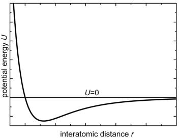
of the molecule as a whole do not change its potential energy. So, we

have U(r1, r2) = U(│r1 – r2│) = U(r), where r = │r1 – r2│. The U(r) function is schematically presented in Fig. 2. For very short interatomic

distances (small r values) the strong repulsion is observed. The repulsion is replaced by attraction for the longer distances (larger r values).

The curve presented in Fig. 2 can be fitted by analytical function, for example, in the form proposed by Lennard-Jones:

where a and b are fitting parameters, which can be derived from the experimental data. This potential is usually used for the description of noncovalent interaction, but we expand it here to covalent bonding for simplicity.

Fig. 1. Maximal durations of the processes

available for the MD simulations using different interatomic potentials

Exercise 2. Please choose the type of potential function U (empirical, semi-empirical or ab initio) which is suitable for MD simulations for the following processes: 1) high-temperature decay of the C60 fullerene, if its lifetime is estimated to be 10 ns; 2) high-frequency oscillation

of the carbon nanotube, if the nanotube is represented by the C1800 cluster and the period of oscillation is about 100 ps; 3) laser-induced isomer-

ization of the allene C3H4, if the reaction proceeds for 10 ps.

8

Exercise 3. Let us assume that the time required for the simulation of the system consisting of N atoms is proportional to Nβ. Using Fig. 1, please estimate the β value for the empirical, semi-empirical and ab initio potentials.

Fig. 2. Potential energy U of two-atomic interaction as a function of the interatomic distance r

Exercise 4. A. Please define in what units are parameters a and b measured, if the molecular system of units is used? B. Experiments show that in the equilibrium at low temperatures, interatomic distance in hydrogen molecule is equal to 0.741 Å, and its energy in this state is equal to 4.75 eV. Using this data, please define the values of a and b parameters in the formula (1).

Exercise 5. Using the values of a and b parameters obtained in Ex. 4, please define the frequency of small oscillations of the H2 molecule. The frequency defined should be compared with the experimental value, which is equal to 4401 cm-1. Try to explain the observed disagreement. Try to propose another two-parametric fitting function instead of (1) providing the calculated oscillation frequency closer to the experimental value.

9

Hydrogen molecule: Tight-binding approach

Calculations based on the empirical potential functions like (1) cannot provide high accuracy if the nonequilibrium states of the system are not taken into account in the fitting procedure, and one needs to study these states. In this case, more accurate description of the interatomic interaction is required. In other words, one needs to use the higher level of theory. Here we consider the tight-binding method. It belongs to the class of semi-empirical methods. In this approach, the potential function U is defined as a sum of two terms:

where Up–p is the proton-proton repulsion, and Uel is the energy of two electrons occupying the lowest one-electron orbital (we consider that the energy does not depend on the spin direction for simplicity). The energy of this orbital can be defined from the one-electron Schrödinger equation for the electron wave function in the field of two protons. The electron wave function is represented as a superposition of two atom-

Exercise 6. Write down the one-electron Schrödinger equation for the wave function expressed in the form (3). Using ( 1 , 2 ) as the basis set, write down the 2 2 matrix of the Hamiltonian operator. Matrix element 1 H 2 should be parameterized as

where h and k are the fitting parameters. Please solve the matrix equation obtained.

data from Ex. 4, please define the fitting parameters h and k. To solve the transcendental equations one can use any mathematical program package or hand-made program.

Exercise 8. Using the h and k parameters obtained in Ex. 7, please define the frequency of the hydrogen molecule small oscillations. The obtained frequency should be compared with the experimental value mentioned in Ex. 5.

10