

ИЭ / 6 семестр (англ) / Лаба / Homework_1_(Electrostatics)_What_to_do
.pdf-The boundary conditions on both symmetry axes. Please note that the boundary conditions on the X-axis and on the Y-axis are not the same. Please think carefully about them.
2.5.CONTROL THE MESH DENSITY
Save again your work and try to build a finite element mesh. The very initial mesh is generated fully automatically by clicking the Build Mesh button on the model toolbar.
The quality of the initial non-controlled mesh should be estimated later. For the first approach it is good enough to get a field solution and validate correctness of the model.
Later, performing the investigation of the dependency of maximal electric field EMAX on the mesh spacing you will use the initial mesh as a starting point and gradually decrease the spacing, increasing the number of mesh nodes.
How to manually control the mesh density:
11
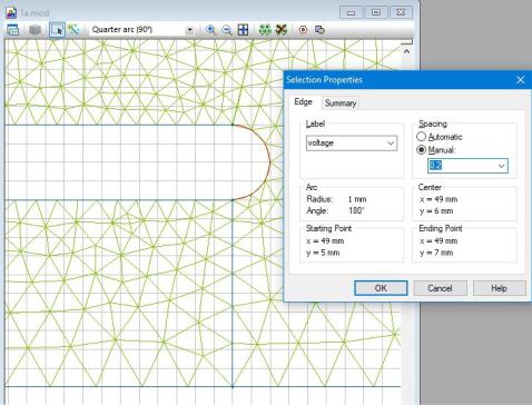
1.Select the object of interest – a block(s), an edge(s) or a vertex (es).
2.Activate the property dialog (Alt+Enter or double click to selected shapes)
3.In the dialog appears switch spacing mode from Automatic to Manual and set the size you want into the input field below.
4.Alternatively, you can switch to Manual mode and enter the spacing value in the Property window that in normally located on the left side below the problem window(s).
When you set some small spacing in the area of interest, do not forget to assign some much bigger spacing to the outer boundary. It is absolutely necessary to avoid over-dense mesh:
12
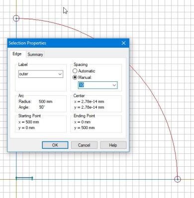
2.6.CHANGE THE RADIUS OF THE ARTIFICIAL OUTER BOUNDARY
The artificial outer boundary is introduced to make the theoretically infinite model bounded. This is needed because QuickField cannot solve an unbounded problem. The requirements for the shape and size of the artificial boundary is to locate far enough from the area in interest to not affect significantly the calculation results. What is calculation results and what is the exact meaning of the word “significantly” very depends on the problem. In this work we assume that the result is maximal value of electric field EMAX, and significantly means more than 1%.
We introduce some reasonable value of the radius of the outer boundary, say ten times more as the half-width of the capacitor, and then have to prove that this choice meets the requirements. This is the reason for investigation the dependence of EMAX = f(radius).
The picture below shows hot to quickly change the arc radius:
1. Go to the Model editor and select the outer arc.
13
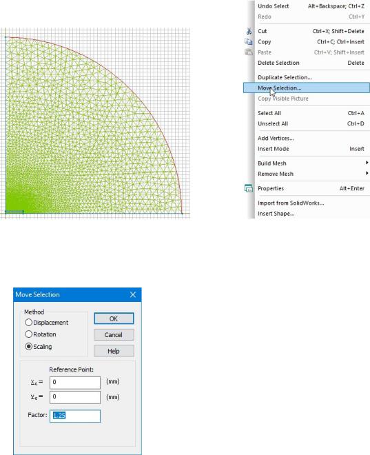
2.In the Edit menu choose Move Selection command
3.In the dialog windows appears choose Scaling and put some scaling factor S > 1
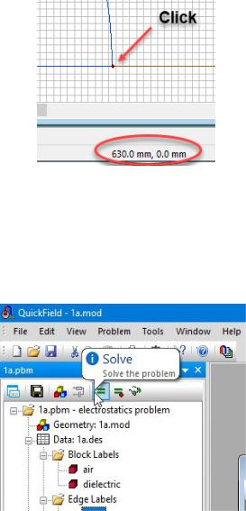
Click OK button and see the new size of the arc. You can measure its new radius by clicking any of two arc corners and watch the coordinates in the status bar (the bottom strip of the QuickField window):
14
2.7.CONTROL THE FIELD PICTURE
Now is a good time to solve your first problem with the default mesh (the mesh with non0controlled spacing). To do that simply click the Solve button on the problem toolbar:
QuickField asks you for saving all modified files, if you didn’t it before, and solves your first problem in a few seconds. The initial field picture appears:
15
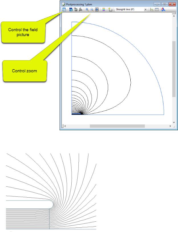
Zoom in to the area of interest – in our study it is the right corner of the capacitor’s plate:
16
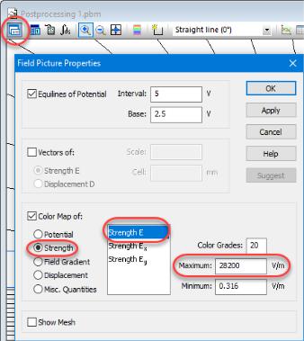
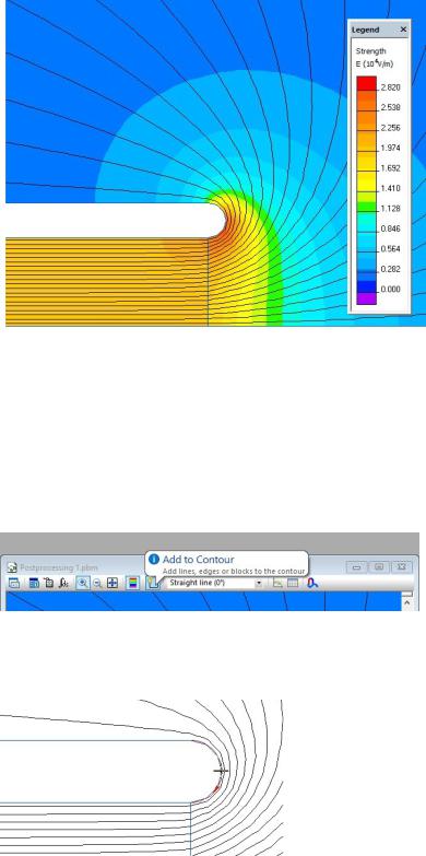
Now tune the field picture to show the color map of E-field magnitude:
To activate the Field Picture Properties dialog, click the leftmost button on the field picture toolbar and in the dialog appears select Color Map and then choose the physical quantity to show – the magnitude of the field strength vector E. The Maximum input field automatically shows you the maximal value of the chosen quantity over the entire model. Now it is E =28.2 kV/m.
17
2.8.XY-PLOT AND TABLE ALONG THE CONTOUR
QuickField can plot and tabulate the field values along the user’s contour. A contour is basically a line or polyline that can be open or closed. The contour consists of one or many parts. Each part is either a free line or a predefined edge of the model.
Let’s build a one-part contour that is simply the semicircular end of the conductor. Enter the contour mode by click to the Add to Contour button
And click by the cross-shaped cursor to the edge of interest:
18
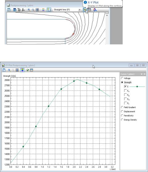
The edge appears in red color with the direction arrow is now the contour suitable for plotting, tabulating and integration. The XY-Plot button brings the XY-Plot, and the Table button opens the window with a field tabulated over the contour.
On the above picture the XY-Plot button and the XY-plot window are shown. The next button on the same toolbar shows field values along the contour in form of table.
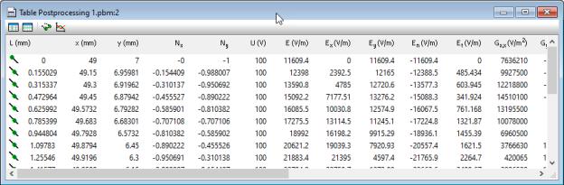
To obtain the maximum electric field value EMAX and the position where the maximal field arises, is recommended to use the table of field values along the contour. By default, the table contains a lot of columns with all known field quantities, and 21 evenly distributed rows:
19
The two leftmost buttons on the table toolbar allow to control table columns and rows:
20