Учебное пособие 2132

Russian Journal of Building Construction and Architecture

vehicle. An increase in the maximum pressure of the liquid during a linear growth of the pressure in the pneumatics onto the roadway surface indicates more presence of the liquid accompanied by deformation of pores and cracks. An increase in the speed of a vehicle might cause the pressure of the liquid to go up more than is characteristic of the impact force P. All of this might lead to hydraulic breakage of the layers of the material a surfacing is made of and thus more intense wear and tear if moistened .

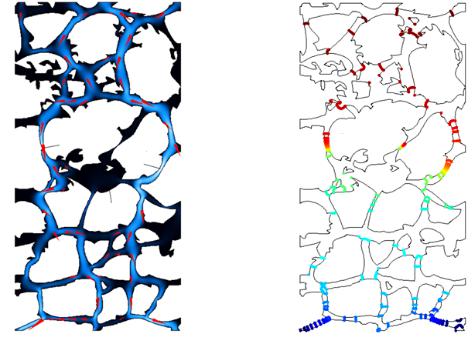
Fig. 4 distinctively shows a non-linear growth of the pressure in the speed range typical of pneumatics impacts. A pressure difference between the upper and lower layer with pores and cracks cause the liquid to start moving.

MPa

P = 300 000Pa

P = 200 000Pa

P = 150 000Pa

m/sec

Fig. 4. Graphs of the dependence of the maximum pressure inside a roadwayelement experiencing failure

and the pressure gradients on the speed of a vehicle

Fig. 5а shows the designed speeds inside the modeled structure and the flow direction. The liquid is known to move with an accelerationin the narrowing channels and even when small, their speed might be as high as 50 and more metres per second. Such a dynamic impact of water results in a significant failure and under certain conditions causes failure with water that in technical literature is referred to as waterjet and is used for shaping and cutting different materials. Due to small speeds failure is lengthy and is [11] about 0,05 mm per hour, which under multiple loading increases the size of defects and thus the porosity of the material with water also contributing to a quick dissolving of non-stable materials. Fig. 5b shows the pressure in the channels of pores and microcracks associated with the hydraulic pressure occurring in these areas. The pressure distribution shows that the particles (besides the hydraulic pressure) is af-

40

fected by a deforming impact of the resulting flows that seek to increase the volumetric penetrability of the channels, pores and cracks. The shearing force of the thin upper layer of the surfacing also contributes to hydrodeformability of its material, which results in failure of the upper layer of the surfacing if moistened.

0.3m/sec

Fig. 5. Designed values: a) of the speed inside the modeled structure; b) of the pressure in the channels of pores and microcracks

Conclusions. It was found that besides the known and previously described defects wear and tear in roadway surfacing is generated by wheel impact of vehicles if there is any moisture on the surface (water wear and tear). In foreign literature an increase in abrasive wear and tear as a mutual defect in the form of rutting occurs on a moistened roadway surfacing is referred to as waterjet. In order to mitigate a defect in the form of rutting caused by wear and tear in asphalt concrete for materials employed in the construction of roadway surfacing, it is necessary that their water resistance is improved and water is quickly drained offthe surfacing if moistened.

A dynamic impact of water moving under a rolling vehicle wheel on the asphalt concrete surfacing is complex and modeling it involves the analysis of the structure of an asphalt concrete. For a more profound insight into the physics of the process a series of natural experiments is essential for a precise evaluation of a dynamic impact of water on an asphalt concrete roadway surfacing and waterjet.

41

Russian Journal of Building Construction and Architecture

References

1.Biderman V. L., Guslitser R. L., Zakharov S. P. Avtomobil'nye shiny [Automobile tire]. Moscow, Goskhimizdat Publ., 1963. 384 p.

2.Korsunskii M. B. Otsenka prochnosti dorog s nezhestkimi odezhdami [Strength evaluation of roads with nonrigid clothes]. Moscow, Transport Publ., 1966. 153 p.

3.Mel'kumov V. N., Matvienko F. V., Kanishchev A. N., Volkov V. V. Prognozirovanie velichiny neobratimoi deformatsii dorozhnoi konstruktsii ot vozdeistviya transportnogo potoka [Prediction of the irreversible deformation of the road structure from the impact of traffic flow]. Nauchnyi vestnik Voronezhskogo GASU. Stroitel'stvo i arkhitektura, 2010, no. 3, pp. 81—92.

4.Nikolaevskii V. N., Basniev K. S., Gorbunov A. T., Zotov G. A. Mekhanika nasyshchennykh poristykh sred

[Mechanics of saturated porous media]. Moscow, Nedra Publ., 1970. 333 p.

5. Nikolaevskii V. N., Livshits L. D., Sizov I. A. [Mechanical properties of rocks. Deformation and fracture].

Itogi nauki i tekhniki. Ser. Mekhanika deformiruemogo tverdogo tela [Results of science and technology. Series Of solid mechanics], 1978, vol. 11, pp. 123—250.

6. Nikolaevskii V. N., ed. Opredelyayushchie zakony mekhaniki gruntov: per. s angl. [Defining laws of soil mechanics]. Moscow, Mir Publ., 1975. 231 p.

7. Abo-Qudais S., Shatnawi I. Prediction of bituminous mixture fatigue life based on accumulated strain. J. Constr. Build. Mater, 2007, vol. 21, pp. 1370—1376.

8.Arabani M., Mirabdolazimi S. M., Sasani A. R. The effect of waste tire thread mesh on the dynamic behaviour of asphalt mixtures. J. Constr. Build. Mater, 2010, vol. 24, pp. 1060—1068.

9.Fontes L. P. T. L., Trichês G., Pais J. C., Pereira P. A. A.Evaluating permanent deformation in asphalt rubber mixtures / L. P. T. L. Fontes, 2010, vol. 24, pp. 1193—1200.

10.Leng J. Characteristics and Behavior of Geogrid-Reinforced Aggregate under Cyclic Load: A Dissertation… for the Degree of Doctor of Philosophy, 2002. 152 p.

11.Louis Н., Pude F., Rad von Ch. Potential of Polymeric Additives for the Cutting Efficiency of Abrasive Waterjets. Proceedings of the 2003 Waterjet Conference, August 17—19, 2003. Houston, TX, 2003. WaterJet Technology Association (WJTA) and Industrial & Municipal Cleaning Association (IMCA). Available at: https://www.wjta.org/images/wjta/Proceedings/proceedings%202003.pdf.

12.Mantzos L., Carpos P., Papandreou V., Tasios N. European energy and transport: trends to 2030: update 2005. Belgium: European Commission. Europe's energy portal. Available at: https://www.energy.eu/publications/KOAC07001ENC_002.pdf.

13.Mahrez A., Karim M. R., Katman H. Y. Fatigue and deformation properties of glass fiber reinforced bituminous mixes. J. Eastern Asia, Soc. Trans. Stud., 2005, vol. 6, pp. 997—1007.

14.Moghaddam T. B., Karim M. R., Abdelaziz M. A review on fatique andrutting performance of asphalt mixes. Scientific Research and Essays, 2011, vol. 6 (4), pp. 670—682.

15.Werkmeister S. Permanent deformation behaviour of unbound granular materials in pavement constructions: PhD thesis. Dresden, Germany, University of Technology, 2003. 189 p.

42

DOI 10.25987/VSTU.2019.42.2.005

UDC 625.08:625.42:681.5

V. A. Medvedev1, V. L. Burkovskii2, V. A. Trubetskoi3, A. K. Mukonin4

THE ROBOT WITH THE ANGULAR COORDINATE SYSTEM

FOR INSTALLATION OF SLEEPERS IN THE METRO

Voronezh State Technical University

Russia, Voronezh

1PhD in Engineering, Assoc. Prof. of the Dept. of Electric Drive, Automation and Control in Technical Systems, tel.: (473) 243-77-20, e-mail: va.medved60@yandex.ru

2D. Sc. in Engineering, Prof., Head of the Dept. of Electric Drive, Automation and Control in Technical Systems, Honored scientist of the Russian Federation, tel.: (473) 243-76-87, e-mail: bvl@vorstu.ru

3PhD in Engineering, Assoc. Prof. of the Dept. of Electric Drive, Automation and Control in Technical Systems, tel.: (473) 243-77-20

4PhD in Engineering, Assoc. Prof. of the Dept. of Electric Drive, Automation and Control in Technical Systems, tel.: (473) 243-77-20

Statement of the problem. The article deals with the questions of designing of the manipulation robot for the installation of sleepers in the metro. To reproduce the required trajectories at high speeds of movement of the manipulator links, the task is to develop its dynamic model, as well as the structure of the microprocessor system of dynamic control of the manipulator.

Results. The equations of dynamics of a three-coordinate manipulator with an angular coordinate system in the differential and vector form of recording, providing the solution of the inverse problem of dynamics, are obtained. The structure of the microprocessor system of dynamic control by three-link manipulator with angular coordinate system is developed.

Conclusions. It is advisable to use three-coordinate manipulators with an angular system of coordinate in a limited space of the metro. At formation of control actions on the drives of the robot for installation of sleepers is rational to use a method of dynamic control, developing a dynamic model of the manipulator based on its design scheme and the Lagrange method.

Keywords: robot for installation of sleepers, manipulator, dynamic model, dynamic control, angular coordinate system.

Introduction. Operational and reliability requirements for metro s are rather demanding. However, features of metro (small sizes of tunnels, contact sleepers and short nighttime technological “slots”) curb the use of equipment and construction techniques employed for track maintenance and repairs.

© Medvedev V. A., Burkovskii V. L., Trubetskoi V. A., Mukonin A. K., 2019

43

Russian Journal of Building Construction and Architecture

As track maintenance in a tunnel is restricted in time and labour-intensive, developing heavyduty manipulative robots and reducing labour costs is not only a technical but also a social issue that needs to be addressed. It is advisable to use three-coordinate manipulators with an angular coordinate system that are compact and can thus be folded, which is an essential consideration for enclosed metro spaces.

The characteristics and parameters of manipulation robots are determined by their technological performance as well as certain implementations of their operational systems. A microprocessor implementation of an operational system with an angular coordinate system allows an almost two-time reduction in energy costs in a system designed using low and medium integration scale microschemes [11].

A reduction in times of track maintenance in tunnels depends on improving the performance of employed manipulation robots. For high-quality development of required routes for highspeed chains of a manipulator, a dynamic should be introduced into its operating system for a inverse dynamics task [9, 12, 13].

Therefore in order to design a robot for laying metro sleepers , it is necessary that a dynamic model of a three-coordinate manipulator with an angular coordinate system is developed for a inverse dynamics task as well as a structure of a microprocessor system of a dynamic operational system of a manipulator.

1. Methods of designing a dynamic model. A robot’s handles should be operated at a high frequency (no less than 50 Hz) asthe resonance frequency of manipulators is about 10Hz. Real-time calculations no less than each 20 msec call for modern computing machines with a few processors necessary for operating manipulators under certain conditions. Therefore let us look at a number of solutions for a direct and inverse dynamics task from the viewpoint of minimizing a number of calculations for designing a dynamic model.

The first result that was employed for a direct as well as a inverse dynamics task was obtained by Walker by means of Lagrange’s method [19]. Kahn [17] developed an algorithm for modeling disconnected kinetic chains. Jang [21] implemented the method in a software for analyzing the dynamics of robots. Hollerbach [16] showed that the number of multiplication/sum operations used in these methods depends on n4 (n is the number of degrees of freedom) and for manipulators with three degrees of freedom there should be 5.000 multiplications and around the same number ofsums. These methodsare implemented in realtime by modern high-speed computers. Waters and Hollerbach developed algorithms for solving only an inverse dynamics task based on the Kahn-Walker method. The number of multiplication/sum operations in these algo-

44

rithms was reduced to that proportionate to n [16]. However, in this case 1.000 multiplications are required for three-coordinate manipulators.

In [8] a dynamic model of the manipulator “PUMA-560” designed using the Newton-Euler method in the MATLAB environment is discussed. The Newton-Euler method allows a dynamic model to be designed with a random coordinate system [7], i.е. they are universal. One of the downsides of the Newton-Euler method is that in order to identify the kinetic parameters of the chains of the manipulator at each discrete interval for designing operations in realtime, the coordinates have to be transformed.

Let us point out the property that all of the above methods share. They do not depend on a type of a kinetic scheme of the manipulator and rely on the general kinetic laws and solid body dynamics. For a manipulator with a certain kinetic scheme designing an analytical model requires fewer arithmetical operations. This is proved in [17, 20]. Designing a model of an anthropomorphic three-coordinate manipulator requires no more than 44 multiplications and 23 sums. For a manipulator with five degreesof freedom a totalof 352 multiplications are needed [18].

Hence for operating manipulators in real-time, it is viable to make use of the methods aimed at particular kinetic schemes for the sake of saving hardware and software tools. Therefore a dynamic model of a three-coordinate manipulator with an angular coordinate system will be designed using its calculations scheme with the aid of the Lagrange tool [4].

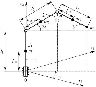
2. Developing a dynamic model with an angular coordinate system. A calculation scheme of a three-coordinate manipulator with an angular coordinate system is given in Fig. 1.

Fig. 1. Calculation scheme of the manipulator with an angular coordinate system

45

Russian Journal of Building Construction and Architecture

The chain 1 has the mass m1 and inertia moment J1 in relation to the rotation axis Оx2. Using m2, m3 and m the mass of the chains 2, 3 respectively and the operating body are designated. The lengthofthe chains isdesignated asl1, l2, l3,the distance fromthe centresofthe massesm1, m2, m3 to the joining centres as l01, l02, l03. The manipulator in question has three rotating kinetic pairs. A vector of the generalized coordinates of the manipulator consists of the rotation angles at the joining chains1, 2, 3:q = [ 1, 2, 3]. Fig. 1 also showsa Cartesian coordinate system0x1x2x3.

While designing a dynamic model of the manipulator with an angular coordinate system let us assume that the parameters of the chains of the manipulator (length, mass, inertia moments, etc.) are known and can be considered constant. The joining coordinates (angles or linear movements of the chains) and their derivatives will be considered independent variables. All the other values used for designing the mathematical models will be viewed as the functions of the joining coordinates (generalized coordinates of the manipulator).

The Lagrange equations for the three-coordinate manipulator are asfollows:

where W is the kinetic energy of the manipulator; П is the potential energy of the manipulator;

M j are the moments developed by the electric conductors in the rotating joints.

The chain 1 is only involved in the rotation along the coordinate 1. Hence its kinetic energy is given by the expression

The chains 2 and 3 move in a complex manner. Let us denote the linear speed of the points where the mass m2, m3 and m is concentrated as V2, V3 and V. Then to determine the kinetic energy of the chains 2, 3 and load m let us write the following expressions:

The square of the speed of the point m2 is identified using the equation:

The Cartesian coordinates xs3 of the point m3 are given by the expression:

x13 [l2 cosφ2 l03 cos(φ2 φ3)] sinφ1;

x33 [l2 cosφ2 l03 cos(φ2 φ3)] cosφ1.

46

Differentiating the coordinates xs3 using the time we get:

x33 [l2φ2 sinφ2 l03(φ2 φ3) sin(φ2 φ3)] cosφ1 [l2 cosφ2l03 cos(φ2 φ3)] sinφ1φ1.

The square of the speed of the point m3 is

(7) Inserting (7) the expressions for determining the speedx13 , x23 and x33 from (6) into (7), following a series of trigonometry transformations we get the following equation:

Similarly the following expression for the square of the speed of the point m is deduced:

The kinetic energy W of the manipulator is given by the expression:

Based on the equations (2)—(4), (8)—(10), we get the following expression for the kinetic energy of the manipulator:

m{l22( 12 cos2 2 22) l32[( 2 3)2 12 cos2( 2 3)]

2l2l3[ 2( 2 3)cos 3 12 cos 2 cos( 2 3)]}/2.

The particular derivatives of the kinetic energy of the speed of the generalized coordinates are as follows:

47

Russian Journal of Building Construction and Architecture

The derivatives of the kinetic energyW using the generalized coordinates are the following:

The derivatives of the potential energyП using the generalized coordinates are as follows:

Inserting the expressions for the particular derivatives (12), (13) and (15) into (1), following a series of time differentiations and denotations, we get the following equations of the dynamics of the manipulator with an angular coordinate system:

Bφ1(φ2,φ3,φ1,φ2,φ3) φ1{ (m2l022 ml22 m3l22)sin2φ2 φ2 (m3l032 ml32)sin[2(φ2 φ3)](φ2 φ3) 2l2(m3l03 ml3)[sin(2φ2 φ3) φ2 cosφ2 sin(φ2 φ3) φ3};

Aφ2 (φ3) m2l022 m3l22 ml22 m3l032 ml32 2cosφ3l2(m3l03 ml3);

Bφ2(φ2,φ3,φ1,φ2,φ3) (2φ2 φ3)l2 sinφ3 φ3(m3l03 ml3) φ12{(m2l022 m3l22 ml22)

sin(2φ2) (m3l032 ml32)sin[2(φ2 φ3)] 2(m3l2l03 ml2l3)sin(2φ2 φ3)}/2;

Cφ2(φ2,φ3) g(m2l02 m3l2 ml2)cosφ2 g(m3l03 ml3)cos(φ2 φ3);

Aφ3 m3l032 ml32; Aφ32 (φ3) m3l032 ml32 l2 cosφ3 (m3l03 ml);

48

The vector form of the equation system (16) is

A(q)q+B(q,q)+C(q) = P, (18)

where A(q),q is the matrix of the inertia parameters and column vector of the accelerations;

B(q,q)is a column vector considering the mutual effect of the coordinates; C(q) is a column vector of the gravitational forces; P is a column vector of the generalized forces in the joints of the manipulator.

The matrix A(q) and vectors q , P, B(q,q), C(q) are determined in the following way:

3. Dynamic operation of the manipulator. A mathematical model of the dynamics of the manipulator is immediately included into the structure of the operation system in a dynamic operating system. In [2, 3, 12, 13] an approach is described that involves designing a complete dynamic model in the process of operation, i.e. calculating the vectors of the generalized forces according to the equation (18) using the vectors of the measured generalized coordinates q(t) and speed q(t) of the robot. The robot is asymptomatically stable in the vicinity of the nominal trajectory if the vector of the generalized forces is

where K0 is the matrix sized n n of the coefficients of the inverse position connection based on the position; K1 is the matrix sized n n of the coefficients of the inverse connection based on the speed.

A scheme of designing operating efforts in accordance with (20) is given in Fig.2. The vector P(t) is calculated using the equation (20); the vector I(t) of the operating current flows is calculated based on the vector P(t) considering the parameters of kinetic transmissions. The scheme takes into account the mutual influence of the chains (the matrix B(q,q)), gravitational forces (the matrix C(q)), changes in the inertia moments during movement of the manipulator (in the matrix A(q)).

49