

Учебное пособие 2132
.pdfRussian Journal of Building Construction and Architecture
where B is an average number of users per 1 km2; s is a specific cost of a financial characteristics; П is a heat density of an area; Δτ is a design fluctuation in the temperatures of a heat carrier; ϕ is a correction coefficient.
Fig. 1 and 2 show changes in an optimal radius of heat supply as a heat energy source shifts due to an increase in a financial characteristics of a network. The figure suggests that as a source is gradually removed from the centre of heat consumption, most remote customers might be outside an optimal radius of heat supply and their costs might thus go up.
Fig. 3. Dependence
of a theoretical and actual moment
of a thermal load
Analysis of existing projects |
|
Analysis of dependencies (7) |
|
|
|
One of the major drawbacks of this method is an empirical character of the applied dependencies that are not always capable of giving a clear understanding of an actual state of affairs in the industry due to changes in the relevant economic laws [5]. E.g., in [1] it is noted that a service area of a source can “cover” the entire area of a city, which is an unlikely thing to do due to a combination of factors. This suggests that these dependencies require correction. Besides, a longer planning of heat supply (see Fig. 2) can be less preferable in terms of even distribution of a thermal load. However, a financial characteristics of similar systems can be lower compared to more compact systems (see Fig. 1).
Conclusions. 1. All of the above suggests that location of functional areas of cities has a direct effect on optimal routing of heat supply networks increasing construction costs as a heat source is removed from the centre of a heat supply area. An optimal radius of heat supply drops making connecting more remote customers not economically feasible.
2. Being semiempirical, existing methods and dependencies individually do not provide a consistent and concise description of heat supply systems. Hence efficiency of the systems should be evaluated based on multiple-criteria optimization methods.
90
Issue № 2 (42), 2019 |
ISSN 2542-0526 |
References
1.Akhmetova I. G. Sistema kompleksnoi otsenki i povysheniya effektivnosti tsentralizovannogo teplosnabzheniya ZhKKh i promyshlennykh predpriyatii. Diss. d-ra tekhn. nauk [System of complex estimation and increase of efficiency of district heating of housing and communal services and industrial enterprises. Dr. eng. sci. diss.]. Kazan', 2017. 331 p.
2.Mel'kumov V. N., Kuznetsov I. S., Kobelev V. N. Vybor matematicheskoi modeli trass teplovykh setei [The choice of the mathematical model tracks thermal networks]. Nauchnyi vestnik Voronezhskogo GASU. Stroitel'stvo i arkhitektura, 2011, no. 2, pp. 31—36.
3.Mel'kumov V. N., Kuznetsov I. S., Kobelev V. N. Zadacha poiska optimal'noi struktury teplovykh setei [The problem of finding the optimal structure of heat networks]. Nauchnyi vestnik Voronezhskogo GASU. Stroitel'stvo i arkhitektura, 2011, no. 2, pp. 37—42.
4.Mel'kumov V. N., Sklyarov K. A., Tul'skaya S. G., Chuikina A. A. Kriterii optimal'nosti i usloviya sravneniya proektnykh reshenii sistem tep-losnabzheniya [Optimality criteria and conditions for comparison of design solutions of heat supplysystems]. Nauchnyi zhurnal stroitel'stva i arkhitektury, 2017, no. 4 (48), pp. 29—37.
5.Papushkin V. N. Radius teplosnabzheniya. Khorosho zabytoe staroe [Radius of heat supply. Well forgotten old]. Novosti teplosnabzheniya, 2010, no. 9, pp. 44—49.
6.Peters E. V. Gradostroitel'stvo i planirovanie naselennykh mest [Urban planning and human settlement planning]. Kemerovo, Izd-vo KuzGTU, 2005. 163 p.
7.Sennova E. V., Sidler V. G. Matematicheskie modelirovanie i optimizatsiya razvivayushchikhsya teplosnabzhayushchikh sistem [Mathematical modeling and optimization of developing heat supply systems]. Novosibirsk, Nauka Publ., 1987. 219 p.
8.Sokolov E. Ya. Teplofikatsiya i teplovye seti [Heating and heating networks]. Moscow, MEI Publ., 2001.
472p.
9.Sokolov E. Ya. Teplofikatsiya i teplovye seti [Heating and heating networks]. Moscow, Gosenergoizdat Publ., 1963. 360 p.
10.Chuikina A. A., Bokhan A. R., Pokataeva V. V., Kolomiichuk A. R. Zavisimost' material'nykh kharakteristik teplovoi seti ot raspredeleniya nagruz-ki [The dependence of the material characteristics of the heat network on the load distribution]. Gradostroitel'stvo. Infrastruktura. Kommunikatsii, 2018, no. 3 (12), pp. 16—20.
11.Chuikina A. A., Bokhan A. R., Grigor'eva K. A. Issledovanie svyazi material'noi kharakteristik teplovoi seti i momenta teplo-voi nagruzki [Investigation of the connection between the material characteristics of the heat network and the moment of heat load]. Gradostroitel'stvo. Infrastruktura. Kommunikatsii, 2018, no. 4 (13), pp. 9—16.
12.Chuikina A. A., Khamidulina K. A., Soshnikova E. E., Yakovleva M. A. Issledovanie sushchestvuyushchikh zavisimostei dlya opredeleniya material'noi kharak-teristiki teplovoi seti [Investigation of existing dependences to determine the material characteristics of the heat network]. Gradostroitel'stvo. Infrastruktura. Kommunikatsii, 2018, no. 2 (11), pp. 34—41.
13.Aleksashina V. V., Chernyshov Ye. М., Chuykin S. V., Melnikova А. А. The Concept of Redevelopment of the Historical Centre of the Village Kantemirovka, Voronezh Region. Scientific Herald of the Voronezh State Universityof Architectureand Civil Engineering. Construction and Architecture, 2015, no.2 (26), pp. 88—101.
91

Russian Journal of Building Construction and Architecture
14.Mel'kumov V. N., Chujkin S. V., Papshickij A. M., Sklyarov K. A. Modelling of Structure of Engineering Networks in Territorial Planning of the City. Russian Journal of Building Construction and Architecture, 2015, no. 4, pp. 33—40.
15.Mel'kumov V. N., Chuykin S. V., Melnikova A. A. Territorial Planning of Recreational Areas Adjacent to a Residential Development Area. Scientific Herald of the Voronezh State University of Architecture and Civil Engineering. Construction and Architecture, 2016, no. 3 (31), pp. 80—88.
16.Yenin A. Ye , Molodykh M. S. Problems of Architectural Heritage Maintenance by the Example of Country Estates of the Central Chernozem Region. Scientific Herald of the Voronezh State University of Architecture and Civil Engineering. Construction and Architecture, 2010, no. 3, pp. 59—73.
92

Issue № 2 (42), 2019 |
ISSN 2542-0526 |
DOI 10.25987/VSTU.2019.42.2.010
UDC 519.3
O. A. Sotnikova1, N. V. Shchetinin2
MODELLING OF THE DISTRIBUTION OF THERMAL AND CONTAMINANT
POLLUTIONS IN A GROUND LAYER OF URBAN STREETS
Voronezh State Technical University
Russia, Voronezh
1D. Sc. in Engineering, Prof., Head of the Dept. of Designing of Buildings and Structures Named after N. V. Troitskii, tel.: (473)277-43-39, e-mail: ksenija.sotnikova@yandex.ru
2PhD student
Statement of the problem. Due to a sharp lack of free areas particularly in large cities, there is a growth in the number of high rises. There is an overall principle of construction employing compaction of existing residential areas, particularly in central densely populated urban areas. As a result, there are what is called street canyons of giant cities. They accumulate thermal and contaminant pollutions (toxic vapors, aerosols, etc.), which eventually lead to a significant environmental degradation. Mathematical modeling allows the dynamics of changes in the air quality in a layer adjacent to the ground to be predicted in street canyons and to be instantlycontrolled.
Results. The corrected image of the mathematical model of flowing of air flows in urban street canyons was proposed to enable a simpler numerical solution while predicting the dynamics of change in the air qualityin a ground layer.
Conclusions. Calculations using the suggested equations of the mathematical model would allow quicker prediction with no use of complex super-power software.
Keywords: wind flow, ground layer of the atmosphere, pollution sources, modeling.
Introduction. Local distribution of pollution in the lower atmospheric layer of city streets largely depends on thermal dynamic parameters of the atmospheric boundary layer, from a geometric configurationof buildings, their mutual position and that ofheat sources(or pollution).
This have a major effect on an overall pattern of air flows (a qualititative characteristics). Therefore in order to predict turbulization of air flows and a relevant pattern of heat/pollution distribution in the ground atmospheric layer ofcity streets for active management by means of pollution emission or justifying the position of air inlets or vents, all flow fields should be modeled with the greatest level of precision [1—7].
© Sotnikova О. А., Schetinin N. V., 2019
93
Russian Journal of Building Construction and Architecture
1. Use of mathematical modeling for describing aerodynamics processes of air flows in-
side city quarters. Let us assume that major similarity parameters determining physical phenomena (the Reynolds and Grashof number) are crucial in this kind of tasks and are way over the critical ones that are typical of a turbulent mode. Therefore in order to be able to predict better, a mathematical model of air flows in city street canyons should be improved, i.e. a reliable solution model for big Reynods and Grashof numbers should be in place.
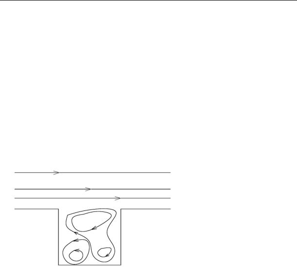
The authors of [5] looked at this problem (obtaining stable and sufficienly accurate numerical solutions for flow fields with high reverse flow rates) where they dealt with a flow in a boundary layer over a wall with a rectangular cave (Fig. 1). Here the heat sourcr placed at the bottom of the cave models heat/pollution emission generating upstream flows that interacting with the main flow ofthe “blown” air mass (Fig. 1).
Fig. 1. For the model described in [5]
It should be noted that a thermally and orographically heterogeneous underlying surface generates special features of air mass movement (and thus pollution distribution) in the ground atmospheric layer. The wind speeds in the vicinity to the ground can get extremely large with some areas where the concentration of pollutants is significantly higher than their values over a horizontal, thermally homogeneous underlying surface under identical conditions.
It is only mathematical modeling that is capable of giving some insight into flow distribution for an infinite variety of landscapes. It might turn out particularly beneficial to emply mathematical model for emergency heat/pollution emission inside densely populated city quarters. Here the use of physical modeling seems extravagant and interpretation of results obtained using a physical model in actual city quarters might get tricky (particularly because of the “large-scale effect”). For landscape planning and preliminary analysis of an area it is more sensible to carry out a series of numerical calculations using the model and employ physical modeling only when it is absolutely necessary.
94
Issue № 2 (42), 2019 |
ISSN 2542-0526 |
Currently for mathematical modeling of atmospheric processes over a complex underlying surface three-dimensional models are commonly used [5—7]. They are quite indicative of the influence of a variety of factors on air movement and heat and air flow distribution in the ground layer of a complex surface. However, for calculations with a high spatial dimesion of a dependence the solutions obtained while using three-dimensional models require highperformance computing machines with an option taking a great deal of time to implement.
Mathematical modeling is commonly used as a supplement of the result of natural measurements of thermal dynamic and concentration parameters and allows one to predict the above values in the space between the points of natural measurements. Therefore developing and studying more simple models of atmospheric aerodynamics in the ground layer and pollution transfer over a complex underlying surface is an urgent issues that needs extra effort to address.
2. Mathematical statement of the problem. For numerical modeling throughtout [5] the Navier-Stock equation was used that was simplified using the Boussinesq approximation. For otiginal functions the initial equations are
u |
|
w |
|
|
Gr T |
|
|
|
1 |
|
2 |
|
|
|
2 |
, |
(1) |
||||||||||||||||||||||||||
|
|
|
|
|
|
|
|
|
|
|
|
|
|
|
|
|
|
|
|
|
|
|
|
|
|
|
|
|
|
|
|
|
|
|
|
|
|
||||||
t |
x |
|
z |
|
|
|
Re |
2 |
|
|
|
|
|
|
2 |
|
x |
2 |
|
|
z |
2 |
|||||||||||||||||||||
|
|
|
|
|
|
|
|
|
|
x Re |
|
|
|
|
|
|
|
|
|
|
|
|
|||||||||||||||||||||
|
|
T |
|
|
uT |
|
|
wT |
|
|
1 |
|
|
|
|
|
2 |
|
|
|
|
2 |
|
|
|
|
|
|
|
||||||||||||||
|
|
|
|
|
|
|
|
|
|
T |
|
|
T |
, |
|
|
|
(2) |
|||||||||||||||||||||||||
|
|
|
|
|
|
|
|
|
|
|
|
|
|
|
2 |
2 |
|
|
|
|
|||||||||||||||||||||||
|
|
t |
x |
|
|
|
|
z |
|
|
|
|
RePr |
|
x |
|
z |
|
|
|
|
|
|
|
|||||||||||||||||||
|
|
|
|
2 |
|
|
2 |
|
|
|
|
|
|
|
|
|
|
|
|
|
|
|
|
|
. |
|
|
(3) |
|||||||||||||||
|
|
|
|
|
|
|
|
|
|
|
, |
|
u |
|
|
|
, |
|
|
w |
|
|
|
|
|
||||||||||||||||||
|
|
2 |
|
|
z |
2 |
|
|
|
|
|
|
|
|
|
x |
|
|
|||||||||||||||||||||||||
|
|
|
|
x |
|
|
|
|
|
|
|
|
|
|
|
|
|
|
z |
|
|
|
|
|
|
|
|
|
|
|
|
|
|
|
|||||||||
The equations are written in the dimensionless and traditional form with the following denotations:
Gr g 0L³ H 0 /v2, Pr v/ K, Re U L /v.
A homogeneous nonperturbed flow was taken as an initial condition. For a numerical solution the boundary of a design calculation area was assumed to be as further away from a perturbation area as possible. As a result, on the wallthere were the following boundary conditions:
u w 0, T C , T Cs. (4)
Here ∞ and |
are constant temperatures in an unnperturbed flow and a heat/pollution source |
|||||||
respectively; in the left boundary (upstream): |
|
|
|
|
|
|
||
|
u u z , |
|
w |
0, |
T C . |
(5) |
||
|
|
|
|
|
||||
|
|
|
||||||
|
|
x |
x |
|
|
|
||
In the upper boundary:
95

Russian Journal of Building Construction and Architecture
|
u U , |
w 0, |
T C . |
(6) |
||
In the right boundary (downstream): |
|
|
|
|
||
|
w |
0, |
|
0, |
T C . |
(7) |
|
|
|
||||
|
x |
x |
|
|
||
Generally for the right boundary the boundary conditions are identical (5):
u u x , |
|
w |
, |
T C . |
(8) |
||
|
|
|
|
||||
|
|
||||||
|
x |
x |
|
|
|
||
A simplifying transformation of the original equations (1)—(3) was conducted by using a finite difference scheme and a stationary solution for Gr = 106 and Re = 104 was yielded by the numerical solution. In this case induced convection caused by the motion of the boundary layer over the rectangular cave dominates the natural convection of the heat/pollution source. The reverse flow area existing outside the cave is stable and does not have a significant influence of the external flow.
Thus the entire flow field quicklyreaches a stationary condition with no physical instabilities. If Re = 103 and Gr = 106, the heat/pollution source generates a double area of the reverse flow inside the rectangular cave, which is characteristic of natural convention. At early stages of the process the reverse flow area does not leave the cave but then it expands and starts having a stationary effect on the main “blown” air mass flow. A stationary condition will also be reached after a certain time period but before it does, most of the flow will reach the cave.
It was finally shown that at Re = 102 and Gr = 106 a stationary condition is not possible to achieve and the reverse flow area increases dramatically considerably influencing the process. In the suggested solution of the equations (1)—(3) we have four unknown values. In order to simplify the mathematical model [5] and reducing the number of the unknown values let us transform the equations in the following way. First let us accept the following denotations which are slightly different from those in [5], i.e.: ω is a vortex; ψ is a current function; x, z are the coordinates across and up the street; u, w are the wind speeds across and up the street. Then the initial equations (1)—(3) will take the following form:
|
|
(u ) |
(w ) |
Gr T |
|
1 2 |
2 |
; |
(9) |
|||||||||||||||||||||
|
|
|
|
|
|
|
|
|
|
|
|
|
|
|
|
|
|
|
|
|
|
|
|
|
|
|
|
|
||
t |
|
|
|
|
|
|
|
|
|
|
|
|
x |
2 |
|
z |
2 |
|||||||||||||
|
|
x |
|
z |
Re x |
|
Re |
|
|
|
|
|
|
|
||||||||||||||||
|
T |
|
(uT) |
|
(wT) |
|
|
1 |
|
|
2 |
|
|
|
2 |
|
|
|
|
|
|
|||||||||
|
|
|
|
|
|
T |
|
T |
|
; |
|
|
(10) |
|||||||||||||||||
|
t |
|
|
|
|
2 |
2 |
|
|
|||||||||||||||||||||
|
|
x |
|
|
z |
|
|
|
|
RePr |
x |
|
|
|
z |
|
|
|
|
|
|
|||||||||
96
Issue № 2 (42), 2019 |
ISSN 2542-0526 |
|
|
|
|
|
|
|
|
|
|
|
|
|
|
|
|
|
|
|
|
|
|
|
|
|
|
|
|
2 |
2 |
|
u |
|
|
w |
|
|
|
|
|
|
|
|
|
|
|
|
|
|
|
|
|
|
|
|
|
|
|
|
||||||||||||||||||||||||||||||||||||||||||||||||||||||||||||||||||
|
|
|
|
|
|
|
|
|
|
|
|
|
|
|
|
|
|
|
|
|
|
|
|
|
|
|
|
|
|
|
|
|
|
|
|
|
|
|
|
|
, |
|
|
|
|
|
|
|
|
|
|
|
, |
|
|
|
|
|
|
|
|
|
|
. |
|
|
|
|
|
|
|
|
|
|
|
|
|
|
|
|
|
|
|
|
|
|||||||||||||||||||||||||||||||||||||||
|
|
|
|
|
|
|
|
|
|
|
|
|
|
|
|
|
|
|
x |
2 |
|
|
z |
2 |
|
|
|
|
|
|
|
|
|
|
|
x |
|
|
|
|
|
|
|
|
|
|
|
|
|
|
|
|
|
|
|
|
|
|||||||||||||||||||||||||||||||||||||||||||||||||||||||||||||||||||
|
|
|
|
|
|
|
|
|
|
|
|
|
|
|
|
|
|
|
|
|
|
|
|
|
|
|
|
|
|
|
|
|
|
|
|
|
|
|
|
|
|
|
|
|
|
|
|
|
|
|
|
|
|
|
|
|
|
z |
|
|
|
|
|
|
|
|
|
|
|
|
|
|
|
|
|
|
|
|
|
|
|
|
|
|
|
|
|
|||||||||||||||||||||||||||||||||||||
In the stationary case (see above): |
|
|
|
|
|
|
|
|
|
|
|
|
|
|
|
|
|
|
|
|
|
|
|
|
|
|
|
|
|
|
|
|
|
|
|
|
|
|
|
|
|
|
|
|
|
|
|
|
|
|
|
|
|
|
|
|
|
|
|
|
|
|
|
|
|
|
|
|
|
|
|
|
|
|
|
|
|
|
|
|
|
|
|
|
|
|
|
|
|
|
|
|
|
|
||||||||||||||||||||||||||||||
|
|
|
|
|
|
|
|
|
|
|
|
|
|
|
|
|
|
|
|
|
|
|
|
|
|
|
|
|
|
|
|
|
|
|
|
|
|
|
|
|
|
|
|
|
|
0, |
|
|
|
|
|
T |
|
0. |
|
|
|
|
|
|
|
|
|
|
|
|
|
|
|
|
|
|
|
|
|
|
|
|
|
|
|
|
|
|
|
|
|
|
|
|
|
|||||||||||||||||||||||||||||||||
|
|
|
|
|
|
|
|
|
|
|
|
|
|
|
|
|
|
|
|
|
|
|
|
|
|
|
|
|
|
|
|
|
|
|
|
|
|
|
|
|
|
|
|
|
|
|
|
|
|
|
|
|
|
|
|
|
|
|
|
|
|
|
|
|
|
|
|
|
|
|
|
|
|
|
|
|
|
|
|
|
|
|
|
|
|
|
|
|
|
|
|
|
|
|
|
|
|
|||||||||||||||||||||||||||
|
|
|
|
|
|
|
|
|
|
|
|
|
|
|
|
|
|
|
|
|
|
|
|
|
|
|
|
|
|
|
|
|
|
|
|
|
|
|
|
|
|
|
|
|
t |
|
|
|
|
|
|
|
|
|
|
|
|
|
|
|
|
|
|
t |
|
|
|
|
|
|
|
|
|
|
|
|
|
|
|
|
|
|
|
|
|
|
|
|
|
|
|
|
|
|
|
|
|
|
|
|
|
|
|
|
|
|
|
|
|
|
|
|
|
|
||||||||||
Equation 1: |
|
|
|
|
|
|
|
|
|
|
|
|
|
|
|
|
|
|
|
|
|
|
|
|
|
|
|
|
|
|
|
|
|
|
|
|
|
|
|
|
|
|
|
|
|
|
|
|
|
|
|
|
|
|
|
|
|
|
|
|
|
|
|
|
|
|
|
|
|
|
|
|
|
|
|
|
|
|
|
|
|
|
|
|
|
|
|
|
|
|
|
|
|
|
|
|
|
|
|
|
|
|
|
|
|
|
|
|
|
|
|
|
|
|
|
|
|
|
|
|
||||
|
|
|
|
|
|
|
|
|
|
2 |
|
|
|
|
|
2 |
|
|
|
|
|
|
2 |
|
|
|
|
|
|
2 |
|
|
|
|
|
|
|
|
||||||||||||||||||||||||||||||||||||||||||||||||||||||||||||||||||||||||||||||||||||||
|
|
|
|
|
|
|
|
|
|
|
|
|
|
|
|
|
|
|
|
|
|
|
|
|
|
|
|
|
|
|
|
|
|
|
|
|
|
|
|
|
|
|
|
|
|
|
|
|
|
|
|
|
|
|
|
|
|
|
|
|
|
|
|
|
|
|
|
|
|
|
|
|
|
|
|
|
|
|
|
|
|
|
|
|
|
|
||||||||||||||||||||||||||||||||||||||
|
|
|
|
|
|
|
x |
|
|
|
|
|
|
|
|
|
|
|
x |
2 |
|
|
z |
2 |
|
|
z |
|
|
|
|
|
|
|
|
x |
2 |
z |
2 |
|
|
|
|
|
||||||||||||||||||||||||||||||||||||||||||||||||||||||||||||||||||||||||||||||||
|
|
|
|
|
|
|
|
|
|
|
|
z |
|
|
|
|
|
|
|
|
|
|
|
|
|
|
|
|
|
|
|
|
|
z |
|
|
|
|
|
|
|
|
|
|
|
|
|
|
|
|
|
|
|
|
|
|
||||||||||||||||||||||||||||||||||||||||||||||||||||||||||||||||||||
|
|
|
|
|
|
Gr T |
|
|
|
|
|
|
|
|
|
1 |
|
|
|
|
|
2 |
2 |
|
|
|
|
|
|
2 |
2 |
|
|
2 |
|
|
|
|
2 |
|
|
|||||||||||||||||||||||||||||||||||||||||||||||||||||||||||||||||||||||||||||||||||
|
|
|
|
|
|
|
|
|
|
|
|
|
|
|
|
|
|
|
|
|
|
|
|
|
|
|
|
|
|
|
|
|
|
|
|
|
|
|
|
|
|
|
|
|
|
|
|
|
|
|
|
|
|
|
|
|
|
|
|
|
|
|
|
|
|
|
|
|
|
|
|
|
|
|
|
|
|
|
|
|
|
|
|
|
|
|
|
|
|
|
|
|
; |
|
|
|||||||||||||||||||||||||||||
Re |
2 |
|
|
|
x |
|
|
|
|
|
|
|
|
|
x |
2 |
|
|
x |
2 |
|
z |
2 |
|
|
z |
2 |
|
|
x |
2 |
|
|
|
|
|
z |
2 |
|
|
|
|||||||||||||||||||||||||||||||||||||||||||||||||||||||||||||||||||||||||||||||||||
|
|
|
|
|
|
|
|
|
|
|
|
|
|
|
|
|
Re |
|
|
|
|
|
|
|
|
|
|
|
|
|
|
|
|
|
|
|
|
|
|
|
|
|
|
|
|
|
|
|
|
|
|
|
|
|
|
|
|
|
|
|||||||||||||||||||||||||||||||||||||||||||||||||||||||||||||||||
|
|
|
|
|
|
|
|
2 |
|
|
|
|
|
|
2 |
|
|
|
|
|
2 |
|
|
|
|
|
2 |
|
|
|
|
|
|
|
|
|||||||||||||||||||||||||||||||||||||||||||||||||||||||||||||||||||||||||||||||||||||||||
|
|
|
|
|
|
|
|
|
|
|
|
|
|
|
|
|
|
|
|
|
|
|
|
|
|
|
|
|
|
|
|
|
|
|
|
|
|
|
|
|
|
|
|
|
|
|
|
|
|
|
|
|
|
|
|
|
|
|
|
|
|
|
|
|
|
|
|
|
|
|
|
|
|
|
|
|
|
|
|
|
|
|
|
|
|
|
|
|
|
|
|
|
|
|
|
|
|
|
|
|
||||||||||||||||||||||||
|
|
|
|
|
|
x |
z x |
2 |
|
|
z |
|
|
|
|
z |
2 |
|
|
|
z |
|
|
x |
x |
2 |
|
|
|
|
x z |
2 |
|
|
|
|
||||||||||||||||||||||||||||||||||||||||||||||||||||||||||||||||||||||||||||||||||||||||
|
|
|
|
|
|
|
|
|
|
|
|
|
|
|
|
|
|
|
|
|
|
|
|
|
|
|
|
|
|
|
|
|
|
|
|
|
|
|
|
|
|
|
|
|
|
|
|
|
|
|
|
|
|
|
|
|
||||||||||||||||||||||||||||||||||||||||||||||||||||||||||||||||||||
|
|
|
|
|
|
|
|
|
|
|
|
|
|
Gr T |
|
|
|
|
|
|
|
1 |
|
|
|
|
4 |
|
|
|
|
|
|
4 |
|
|
|
|
|
|
|
|
|
4 |
|
|
|
|
|
|
|
|
|
4 |
|
; |
|
|
|
|
|
|
|
|||||||||||||||||||||||||||||||||||||||||||||||||||||||||||||
|
|
|
|
|
|
|
|
|
|
|
|
|
|
|
|
|
|
|
|
|
|
|
|
|
|
|
|
|
|
|
|
|
|
|
|
|
|
|
|
|
|
|
|
|
|
|
|
|
|
|
|
|
|
|
|
|
|
|
|
|
|
|
|
|
|
|
|
|
|
|
|
|
|
|
|
|
|
|
|
|
|
|
|
|
|
|
|
|
|
|
|
|
|
|
||||||||||||||||||||||||||||||
|
|
|
|
|
|
|
Re |
2 |
|
|
|
x |
|
|
|
|
|
|
|
|
x |
4 |
|
|
|
|
2 |
z |
2 |
z |
2 |
x |
2 |
|
|
|
|
|
|
z |
4 |
|
|
|
|
|
|
|
|
|||||||||||||||||||||||||||||||||||||||||||||||||||||||||||||||||||||||||||
|
|
|
|
|
|
|
|
|
|
|
|
|
|
|
|
|
|
|
|
|
|
|
Re |
|
|
|
|
|
|
|
|
|
|
|
|
|
x |
|
|
|
|
|
|
|
|
|
|
|
|
|
|
|
|
|
|
|
|
|
|
|
|
|
|
|
|
|
|
|
|
|||||||||||||||||||||||||||||||||||||||||||||||||||||||
|
2 2 |
|
|
|
3 |
|
|
|
|
|
|
|
2 2 |
|
|
|
|
|
|
|
3 |
|
|
|
2 2 |
|
|
|
|
|
3 |
|
||||||||||||||||||||||||||||||||||||||||||||||||||||||||||||||||||||||||||||||||||||||||||||
|
|
|
|
|
|
|
|
|
|
|
|
|
|
|
|
|
|
|
|
|
|
|
|
|
|
|
|
|
|
|
|
|
|
|
|
|
|
|
|
|
|
|
|
|
|
|
|
|
||||||||||||||||||||||||||||||||||||||||||||||||||||||||||||||||||||||||||||
|
x z |
x2 |
|
z |
|
x3 |
|
|
|
x z |
|
|
z2 |
|
|
|
z |
|
|
x z2 |
|
z x |
x2 |
|
|
x |
|
z x2 |
||||||||||||||||||||||||||||||||||||||||||||||||||||||||||||||||||||||||||||||||||||||||||||||||
|
|
|
|
2 |
2 |
|
|
|
|
|
|
|
3 |
|
|
|
|
Gr T |
|
|
|
|
|
|
1 4 |
|
|
|
|
|
|
|
|
|
|
|
|
4 |
|
|
|
|
|
|
|
4 |
|
|||||||||||||||||||||||||||||||||||||||||||||||||||||||||||||||||||||||||||||
|
|
|
|
|
|
|
|
|
|
|
|
|
|
|
|
|
|
|
|
|
|
|
|
|
|
|
|
|
|
|
|
|
|
|
|
|
|
|
|
|
|
|
|
|
|
|
|
|
|
|
|
|
|
|
|
|
|
|
|
|
|
|
|
|
|
2 |
|
|
|
|
|
|
|
|
|
|
|
|
|
|
|
; |
|
|||||||||||||||||||||||||||||||||||||||||
|
z x z |
2 |
|
|
|
|
|
|
z |
3 |
|
|
|
|
Re |
2 |
|
|
|
|
|
x |
|
|
|
|
|
|
|
|
|
|
|
4 |
|
x |
2 |
z |
2 |
z |
4 |
|
||||||||||||||||||||||||||||||||||||||||||||||||||||||||||||||||||||||||||||||||||
|
|
|
|
|
|
|
|
|
|
|
|
x |
|
|
|
|
|
|
|
|
|
|
|
|
|
|
|
|
|
|
|
|
|
|
|
|
Re x |
|
|
|
|
|
|
|
|
|
|
|
|
|
|
|
|
|
|
|
|
|
|
|
||||||||||||||||||||||||||||||||||||||||||||||||||||||||||||||||
(11)
(12)
(13)
(14)
(15)
|
3 |
|
|
3 |
|
|
|
|
|
3 |
|
|
3 |
|
|
|
|
Gr T |
|
|
|
|
|
1 4 |
|
|
|
|
|
4 |
|
|
|
|
|
4 |
(16) |
|||||||||||||||||||||||||||||||||||||||||||||||||||||||||||||||||||||||||
|
|
|
|
|
|
|
|
|
|
|
|
|
|
|
|
|
|
|
|
|
|
|
|
|
|
|
|
|
|
|
|
|
|
|
|
|
|
|
|
|
|
|
|
|
|
|
|
|
|
|
|
|
|
|
|
|
|
|
|
|
|
|
|
|
|
|
|
|
|
|
|
|
2 |
|
|
|
|
|
|
|
|
|
|
|
|
|
. |
|||||||||||||||||||||||
|
x |
|
x |
2 |
z |
|
z |
3 |
|
|
z |
|
|
|
|
3 |
x z |
2 |
Re |
2 |
|
|
x |
|
|
|
|
|
x |
4 |
|
|
2 |
z |
2 |
|
|
|
z |
4 |
||||||||||||||||||||||||||||||||||||||||||||||||||||||||||||||||||||||
|
|
|
|
|
|
|
|
|
|
|
|
|
|
x |
|
|
|
|
|
|
|
|
|
|
|
|
|
|
|
|
|
|
|
|
Re |
|
|
|
|
|
|
|
|
|
x |
|
|
|
|
|
|
|
|
|
|
|||||||||||||||||||||||||||||||||||||||||||||||||||||||
Or: |
|
|
|
|
|
|
|
|
|
|
|
|
|
|
|
|
|
|
|
|
|
|
|
|
|
|
|
|
|
|
|
|
|
|
|
|
|
|
|
|
|
|
|
|
|
|
|
|
|
|
|
|
|
|
|
|
|
|
|
|
|
|
|
|
|
|
|
|
|
|
|
|
|
|
|
|
|
|
|
|
|
|
|
|
|
|
|
|
|
|
|
|
|
|
|
|
|
|
|
|
|
|
|
|
|
|
|
|
|
|
|
Gr T |
|
|
|
3 |
|
3 |
|
3 |
|
3 |
|
|
|
|
|
|
1 4 |
|
|
|
|
|
|
4 |
|
|
|
|
|
|
4 |
|
(17) |
||||||||||||||||||||||||||||||||||||||||||||||||||||||||||||||||||||||||||||
|
|
|
|
|
|
|
|
|
|
|
|
|
|
|
|
|
|
|
|
|
|
|
|
|
|
|
|
|
|
|
|
|
|
|
|
|
|
|
|
|
|
|
|
|
|
|
|
|
|
|
|
|
|
|
|
|
|
|
|
|
|
|
|
|
|
|
|
|
|
|
|
|
|
|
2 |
|
|
|
|
|
|
|
|
|
|
|
|
|
|
. |
||||||||||||||||||||
|
Re |
2 |
|
|
x |
|
|
|
|
|
|
|
2 |
|
|
|
|
|
|
z |
3 |
|
|
|
|
|
|
x |
3 |
|
x z |
2 |
|
Re |
x |
4 |
|
|
|
2 |
z |
2 |
|
|
z |
4 |
|
|||||||||||||||||||||||||||||||||||||||||||||||||||||||||||||||
|
|
|
|
|
|
|
|
|
x |
x |
|
z |
|
|
|
|
|
|
|
z |
|
|
|
|
|
|
|
|
|
|
|
|
|
|
|
|
|
|
|
|
|
|
|
|
|
x |
|
|
|
|
|
|
|
|
|
|||||||||||||||||||||||||||||||||||||||||||||||||||||||
Equation 2: |
|
|
|
|
|
|
|
|
|
|
|
|
|
|
|
|
|
|
|
|
|
|
|
|
|
|
|
|
|
|
|
|
|
|
|
|
|
|
|
|
|
|
|
|
|
|
|
|
|
|
|
|
|
|
|
|
|
|
|
|
|
|
|
|
|
|
|
|
|
|
|
|
|
|
|
|
|
|
|
|
|
|
|
|
|
|
|
|
|
|
|
|
|
|
|
|
|
|||||||||||||
|
|
|
|
|
|
|
|
|
|
|
|
|
|
|
|
|
|
|
|
|
|
|
|
|
|
|
|
|
|
|
|
|
|
|
|
|
|
|
|
|
|
|
|
|
|
|
|
|
1 2T |
|
|
|
|
|
|
2T |
|
|
|
|
|
|
|
|
|
|
|
|
(18) |
|||||||||||||||||||||||||||||||||||||||||
|
|
|
|
|
|
|
|
|
|
|
|
|
|
|
|
|
|
|
|
|
|
|
|
|
|
|
|
|
|
|
T |
|
|
|
|
|
|
|
|
|
|
T |
|
|
|
|
|
|
|
|
|
|
|
|
|
|
|
|
|
|
|
|
|
|
|
|
|
|
|
|
; |
|
|
|
|
|
|
|
|
|
|
|
||||||||||||||||||||||||||||
|
|
|
|
|
|
|
|
|
|
|
|
|
|
|
|
|
|
|
x |
|
z |
z |
|
x |
|
|
|
|
|
|
|
|
|
|
|
x |
2 |
|
|
|
z |
|
2 |
|
|
|
|
|
|
|
|
|
|
|
||||||||||||||||||||||||||||||||||||||||||||||||||||||||
|
|
|
|
|
|
|
|
|
|
|
|
|
|
|
|
|
|
|
|
|
|
|
|
|
|
|
|
|
|
|
|
|
|
|
|
|
|
|
|
|
|
|
RePr |
|
|
|
|
|
|
|
|
|
|
|
|
|
|
|
|
|
|
|
|
|
|
|
|
|
||||||||||||||||||||||||||||||||||||||||||
|
|
|
|
|
|
|
|
|
|
|
|
|
|
|
|
2 |
|
|
|
|
|
|
|
|
|
T |
|
|
|
|
2 |
|
|
|
|
|
|
|
|
|
|
T |
|
|
|
|
|
1 |
|
|
|
|
|
|
|
2 |
|
|
|
|
|
2 |
|
|
|
|
|
|
|
|
|
|
||||||||||||||||||||||||||||||||||||||
|
|
|
|
|
|
|
|
|
|
|
|
|
|
|
|
T |
|
|
|
|
T |
|
|
|
|
|
|
|
|
|
T |
|
|
T |
|
|
; |
|
|
|
|
|
|
(19) |
||||||||||||||||||||||||||||||||||||||||||||||||||||||||||||||||||
|
|
|
|
|
|
|
|
|
|
|
|
|
|
|
|
|
|
|
|
z |
|
|
|
x |
|
|
|
|
|
|
|
|
|
|
|
|
|
RePr |
2 |
2 |
|
|
|
|
|
|
|
|||||||||||||||||||||||||||||||||||||||||||||||||||||||||||||||
|
|
|
|
|
|
|
|
|
|
|
|
|
|
|
x z |
|
|
|
|
|
|
|
|
|
|
x z |
|
|
|
|
|
|
|
x |
|
|
|
|
z |
|
|
|
|
|
|
|
x |
|
|
|
z |
|
|
|
|
|
|
|
|
|
|
|||||||||||||||||||||||||||||||||||||||||||||||||
|
|
|
|
|
|
|
|
|
|
|
|
|
|
|
|
|
|
|
|
|
|
|
|
|
|
|
|
|
|
|
|
T |
|
|
|
|
|
|
T |
|
|
|
|
|
|
1 |
|
|
|
|
|
|
|
|
|
2 |
|
|
|
|
|
|
|
|
|
2 |
|
|
|
|
|
|
|
|
|
|
|
|
|
|
|
|
|
|
|
|
|
|||||||||||||||||||||||
|
|
|
|
|
|
|
|
|
|
|
|
|
|
|
|
|
|
|
|
|
|
|
|
|
|
|
|
|
|
|
|
|
|
|
|
|
|
|
|
|
|
T |
|
|
|
|
T |
|
. |
|
|
|
|
|
|
|
|
|
|
|
|
|
|
|
|
(20) |
||||||||||||||||||||||||||||||||||||||||||||
|
|
|
|
|
|
|
|
|
|
|
|
|
|
|
|
|
|
|
|
|
|
|
|
|
|
|
|
|
|
|
|
|
RePr |
2 |
|
|
|
2 |
|
|
|
|
|
|
|
|
|
|
|
|
|
|
|
|
|
|||||||||||||||||||||||||||||||||||||||||||||||||||||||
|
|
|
|
|
|
|
|
|
|
|
|
|
|
|
|
|
|
|
|
|
|
|
|
|
|
|
|
|
|
z |
|
|
|
x |
|
|
|
|
x |
|
z |
|
|
|
|
x |
|
|
|
|
|
z |
|
|
|
|
|
|
|
|
|
|
|
|
|
|
|
|
|
|
|
|
|
|||||||||||||||||||||||||||||||||||||
In the first equation the senior derivatives are |
|
|
4 |
|
, |
|
|
|
|
4 |
|
, |
|
|
|
T |
|
, for the solution we need |
||||||||||||||||||||||||||||||||||||||||||||||||||||||||||||||||||||||||||||||||||||||||||||
|
|
x4 |
|
|
|
|
|
|
z4 |
|
|
|
x |
|
|
|||||||||||||||||||||||||||||||||||||||||||||||||||||||||||||||||||||||||||||||||||||||||||||||
|
|
|
|
|
|
|
|
|
|
|
|
|
|
|
|
|
|
|
|
|
|
|
|
|
|
|
|
|
|
|
|
|
|
|
|
|
|
|
|
|
|
|
|
|
|
|
|
|
|
|
|
|
|
|
|
|
|
|
|
|
|
|
|
|
|
|
|
|
|
|
|
|
|
|
|
|
|
|
|
|
|
|
|
|
|
|
|
|
|
|
|
|||||||||||||||||||
97
Russian Journal of Building Construction and Architecture
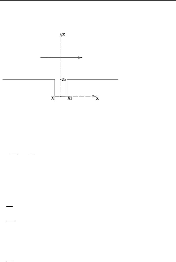
9 boundary conditions. In the second equation the senior derivatives are |
2T |
, |
2T |
, for th |
|
x2 |
z2 |
||||
|
|
|
|||
solution we need 4 boundary conditions (Fig. 2). |
|
|
|
||
Upper boundary
Left boundary |
Wind |
Right boundary |
Fig. 2. Boundaryconditions
for the suggested model
Wall |
Wall |
Wall
The wall:
|
z z0 , |
x x1; |
x x1, 0 z z0 ; |
|
|
z 0, |
x1 x x2 ; |
x x2 , |
0 z z0 ; |
z z0 , |
x x2 . |
1, 2) 0, 0 are projections of the wind speeds onto the axis x and z which are zero;
z x
3)T C is the temperature in the unperturbed flow;
4)T(x*,0) CS is the temperature of the heat/pollution source at z 0; x* is any value in the interval [x1, x2] or a line in this interval.
Here are 4 conditions. The left boundary: z z0 , > ;
5)u(z) is the change function of the wind speed along the height;
z
6)3 3 0;
x
7) T C .
Here are 3 conditions.
The upper boundary: = < ;
8) u* is the established wind speed;
z
98

Issue № 2 (42), 2019 |
ISSN 2542-0526 |
9)0 is the wind speed in the vertical direction;
x
10)T C .
Here are 3 conditions.
The right boundary (similarly to the left one): z z0 , < ;
11)u(z) is the change function of the wind speed along the height;
z
12)3 3 0;
x
13) T C .
Here are 3 conditions.
In [5] for the right boundary another option is proposed:
11)2 0 is a projection of the wind speed onto the vertical along the axis x which is con-
x2
stant;
12) |
|
|
3 |
|
3 |
0 |
is a vortex along the axis х which is constant; |
|
x |
x3 |
x z2 |
||||||
|
|
|
|
|
13) T C .
Therefore the transformations we performed allow us to simply the solution and make the task in hand more definite.
Conclusions. The obtained results are of interest in terms of predicting a pollution pattern of air mass in the ground street spaces (urban street canyons).
Different qualitative flow fields correspond to different wind force and intensity conditions of a heat source (or a pollution source): starting from the option where the air in the ground layer can self-purify by means of dilution and only by diffusion to when a powerful convective flow is joined to the diffusion one. The latter makes it safe to say that the level of hear and contaminant pollution will drop significantly while the quality of the ground atmosphere will benefit greatly.
References
1. Dubinskii S. I. Chislennoe modelirovanie vetrovykh vozdeistvii na vysotnye zdaniya i kompleksy. Avtoref. diss. kand. tekhn. nauk [Numerical simulation of wind impacts on high-rise buildings and complexes. Cand. eng. sci. diss.]. Moscow, MGSU Publ., 2010. 21 p.
99