

Система схемотехнического моделирования Micro-Cap 6.0. Хрестоматия для организации самостоятельной учебной деятельности студентов. Комарова Э.П., Каширский С.Н
.pdfAnimation components
There are three animation components: a digital switch, an LED, and a seven segment display. The description of these are as follows:
Digital Switch: The switch is designed to produce either a digital zero or one state. It has a single output pin at which the selected digital state will appear. During a simulation, the switch may be clicked on to toggle it between its zero and one output. The appearance of the switch's arm will change to indicate which state the switch is currently connected to.
LED: The LED component is designed to represent the display of a light emitting diode. It has a single input pin. Depending on the digital state or the analog voltage at the input pin, the LED will be lit with a different color on the schematic. The colors the LED uses are defined in the Color/Font page of the circuit's Properties dialog box. In this page, there is a list of digital states that have a corresponding color.
Seven Segment Display: The seven segment component is designed to represent the display of a seven segment display. It has an input pin for each segment of the display. All of the pins are active high. It is intended to work with basic seven segment decoders/drivers although any input will control the display of the corresponding segment.
The LED and seven segment display components do not model the electrical characteristics of the parts they represent. They are only available for display purposes. The digital switch is the only one of the three that can effect a simulation. Each of these components must have an I/O model specified for them in order to work with analog components.
Animate Options dialog box
This dialog box sets the interval between data point calculations in an animation analysis. The dialog box is invoked by selecting Animate Options under the Scope menu and appears in Figure 14-1. It provides these options:
108

Wait
Don't Wait: This option turns off the animation which lets the analysis run at optimum speed.
Wait for Key Press: This option will produce one data point with each key press.
Wait for Time Delay: This option will produce one data point per specified time delay.
Time Delay: This text field sets the specified time delay in seconds that will be between each data point calculation. This text field is only active if the Wait for Time Delay option is selected.
OK: This closes the dialog box and saves any changes that were made.
Cancel: This closes the dialog box and ignores any changes that were made.
Help: This accesses the help topic for this dialog box.
Figure 14-1 Animate Options dialog box A transient analysis example
To see how the animation mode works in transient analysis, click on Open under the File menu and load the circuit ANIM3. The ANIM3 circuit uses the seven segment components to display the outputs of three 7448 seven segment decoders. The circuit should appear like this:
109
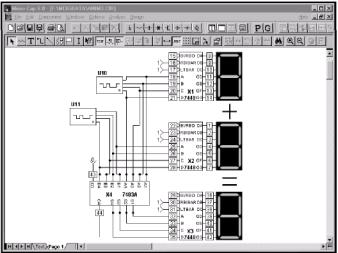
Figure 14-2 The ANIM3 circuit
Select Transient from the Analysis menu. Close the Analysis Limits dialog box. Click on the Scope menu and select Animate Options. The Wait setting for the ANIM3 circuit is currently set to Wait for Time Delay and the Time Delay has been defined as Is. This means that a single data point will be calculated every second. Click OK. Hit the F2 key to run the simulation. Every second a new data point will be calculated. The resulting values will be displayed in the plot and on the schematic. Notice that both the digital states on the schematic and the seven segment displays are updated with each data point. Figures 14-3 and 14-4 display the simulation results at two separate times in the circuit.
For animate mode, a split screen should be used to be able to view both the waveform plot and the schematic at the same time. This can be done by selecting Tile Vertical or Tile Horizontal under the Windows menu. The schematic can be moved within the window by dragging with the right mouse button.
The waveforms in the plot also show the output values of the Ina stimulus (nodes 21-18), the Inb stimulus (nodes 28-25), and the resulting output (nodes 35-32) of the adder. As can be easily seen in the
110

Figure 14-3 Animation mode results at 150ns
figures, it is much easier to view the basic output through the animation components than through the actual waveforms.
Figure 14-4 Animation mode results at 650ns
111
|
Menus |
|
|
|
|
File |
Edit |
Component |
|
|
|
New |
Undo |
Analog Primi- |
Open |
Cut |
tives |
Save |
Copy |
Analog Library |
Save As |
Paste |
Digital Primi- |
Translate |
Clear |
tives |
Revert |
Select All |
Digital Library |
Delete |
Copy Front Window |
Animators |
Close |
Add Page |
Find Component |
Print Preview |
Delete Page |
|
Add Model State- |
|
|
Print Setup |
ments |
|
Exit |
Box Operations |
|
Circuit 1 |
Change |
|
Circuit 2 |
Bring to Front |
|
... |
Send to Back |
|
Circuit N |
Find |
|
|
Repeat |
|
|
Replace |
|
Windows |
Options |
Analysis |
|
|
|
Cascade |
Tools |
Transient Analy- |
Tile Vertical |
Help Bar |
sis |
Tile Horizontal |
Mode |
AC Analysis |
Arrange Icons |
View |
DC Analysis |
Maximize |
Show All Paths |
Probe Transient |
Zoom In |
Preferences |
Analysis |
Zoom Out |
Global Settings |
Probe AC Anal- |
Toggle |
Title Block |
ysis |
Text/Drawing |
Component Palette 1 |
Probe DC Anal- |
Split Horizontal |
Component Palette 2 |
ysis |
Split Vertical |
Component Palette 3 |
|
Show Full Window |
... |
|
|
112 |
|
Component Editor |
Component Palette 9 |
|
Shape Editor |
|
|
Model Program |
|
|
Calculator |
|
|
Tool Bar |
|
|
Transient Analysis |
Scope |
Monte Carlo |
AC Analysis |
|
|
DC Analysis |
|
|
|
|
|
Run |
Remove All Objects |
Options |
Limits |
Restore Limit Scales |
Histograms |
Stepping |
Numeric Format |
|
Analysis Plot |
View |
|
3D Plots |
Cursor Functions |
|
Performance Plots |
Singe Step |
|
Numeric Output |
Go To X |
|
State Variables Edi- |
Go To Y |
|
tor |
Go To Performance |
|
DSP Parameters |
Tag Left Cursor |
|
Reduce Data Points |
Tag Right Cursor |
|
Exit Analysis |
Tag Horizontal |
|
|
Tag Vertical |
|
|
Align Cursors |
|
|
Same Y Scales |
|
|
|
|
113
Symbols
$COMPANY 215 $DATE 215 $MAXPAGE 215 $MAXSHEET 215 $NAME 215 $PAGE 215 $PAGENAME 215 $SHEET 215 $TIME 215 $USER 215
.MODEL 38
.PARAMETERS 199
.SUBCKT 211 3D plots 43
A
AC analysis 107 Accessing 45, 109
Excitation 108 System variables 108
Accel PCB interface 27 Active filters 47
Add model statements command Add page command 30
Adding components 60, 83 Adding tags to plots 144 Adding text to plots 143 Align cursors command 133 Analog library 32
Analog primitives 32, 64 Analog waveforms 8, 15 Analysis Limits dialog
box 8, 86, 110, 123, 124 Command buttons
Add 86, 110, 124 Delete 86, 110, 124 Expand 87, 110, 124 Help 87, 110, 124 Run 86, 110, 124 Stepping 87, 110, 124 Numeric limits field Frequency range 110 Maximum change 111
Index
Maximum time step 87 Noise input 111
Noise output 111
Number of points 87, 110, Temperature 87, 111, 125 Time range 87
Options
Auto scale ranges 90, 114, Frequency step 113 Normal run 89, 113, 127 Operating point 90, 114 Operating point only 90 Retrieve run 89, 113, 128 Save run 89, 113, 128 State variables options Leave 89, 113
Read 89, 113
Zero 89, 113
Animation 48, 155, 223 Components 225 Example 227 Mode 33, 223 Options 226
Arrange icons command 34 Attributes 18, 60
Attribute list box 60 Dialog box 60, 69, 73 Text 19
Text display command 38 Auto scale command 112, 131 Auto scale option 89
B
B field plots 159 Baseline 131 Batch mode 16
Behavioral modeling 1 Bessel filters 47
Border display command 38 Box 18, 30
Bring to front command 31 BSIM models 1
114
C
Calculator 35 Capacitance plots 159 Cascade command 34 Change commands
Attributes 30, 31 Color 31
Font 31 Properties 30
Rename components 31 Charge plots 159 Chebyshev filters 47
Circuit control menu 22 Clear command 29, 74 Click the mouse 18 Clipboard 18
Close command 22, 27 Color menu 88, 112, 127 Command line 16
Command text display command 38 Component
Definition 18 Menu 32
Component Editor Access command 35
Add component command 51, 52 Add group command 52
Adding a new component 50 Copy command 52
Creating pins 20 Delete command 52 Display 50
Display Value / Model Name 51 Merge command 52
Model = Component Name 51 Paste command 52
Pin assignments 51 Pin text option 51
User palette assignment 51 User palette membership 62
Component library 1, 64 Component mode command 36 Condition display command 38 Copy command 18, 29, 75, 83
Copy to clipboard command 29 Copy to picture file command 29 Cross-hair display command 38 Current 7
Current display command 38 Cursor 18
Cursor mode 13, 133, 137, 138 Cursor mode command 37 Cursor value fields 137
Cut command 29, 74, 83
D
Data directory 4 Data entry
Keyboard 25 Mouse 25
DC analysis 45 Default component 83
Default setting for new circuits 42 Define command 6
Delete all objects command 131 Delete file command 27
Delete page command 30 Deleting objects 74 Deselecting objects 76 Design menu 47
DEV tolerances 180 Dialog boxes 25 Digital
Hex operator 7 State 7
Digital library 32 Digital primitives 32, 64 Digital waveforms 8, 15 Drag 18
Drag copying 77, 83 DSP 49
Dynamic DC analysis 12, 45, 48
E
Editing parameters and text 69 Elliptic filters 47
Email for technical support 48 Equipment required 3
115
Esc key 19
Exit command 28 Expressions 7, 8, 13, 91
F
File
Binary model 54 Text model 54 File menu 26 SPICE files 1
Filter designer 49 Filters 33, 47 Find command 31
Find component command 33 Flag mode command 37 Flags 23
Flip X command 30 Flip Y command 30 Fourier analysis 49 Function keys 56
CTRL + F9 Delete all plots 56 F1 Help 56
F10 Properties dialog box 56
F11 Stepping dialog box 56
F12 State Variables editor 56
F2 Run analysis 56
F3 Exit analysis 56
F4 Display analysis plot 56
F5 Display numeric output 56
F6 Auto scale 56
F7 Scale mode 56
F8 Cursor mode 56
F9 Analysis Limits dialog box 56
G
Gaussian distribution 182 Global settings 44, 171 Gmin stepping 40
Graphics mode command 36 Grid 19
Grid text 19
Grid text display command 38
H
H field plots 159 Hardware requirements 3 Help mode command 37 Help System 48 Horizontal tag mode 134
Horizontal tag mode command 37
I
I-V characteristics 123 Inductance plots 159 Inertial cancellation 40 Info mode command 37 Initialization 103 INOISE 118 Installation 4
Inverse-Chebyshev filters 47
L
Linear DC stepping 125 Linear plot option 88 List DC stepping 125 Load MC file 27
Log DC stepping 125 Log plot option 88 LOT 180
LOT tolerances 180
M
Macro
Definition 19, 197 Parameters command 198
Make macro command 30 Maximize command 22, 34 Maximum time step 87 MC6 5
Menus 21 Control 21 Selection 24
Minimize command 22 Mirror box command 30 Mode commands 36 Model Editor
116
Add command 55 Copy command 55 Delete command 55 Go to command 55 Memo field 55 Merge command 55 Pack command 55 Part field 55
Part selector 55 Type Selector 55
Model editor 54 Model library 54
Binary form 54 Text form 54
MODEL program 5, 35, 54 Model statement 64, 69 Monte Carlo
Distributions
Gaussian 182
Uniform 182 Worst case 182 Example 187 How it works 180 Options
Distribution to Use 186 Number of Runs 186 Report When 186 Status 186
Standard deviation 182 Monte Carlo analysis 49 Move command 22
N
Navigating 23, 78, 83, 164 Flagging 78
Paging 78
Panning 78 Relocation 78 Scaling 78 Scrolling 78
New command 26, 83 Next window command 22 Node
Definition 19 Names 19, 67, 83
Numbers 20, 67
Node numbers display command 38 Node snap 68
Node voltages display command 38 Noise
Analysis 118
Flicker 118 Shot 118 Thermal 118
NOM.LIB 30, 208, 212 Normalize command 132 Number of points 87, 110, 126 Numeric output
AC 117
DC 126 Transient 87
Nyquist plots 120
O
Object 20 ONOISE 118 Open command 26 Open model file 54
OrCad PCB interface 27
P
P column 8 Package editor 35 Package library 40 Page
Scroll bar controls 23 Selector tabs 23
Panning 20, 78, 80, 136, 164 Passive filters 47
Paste command 20, 29, 74, 75, 83 PCB interface 1, 26, 35 Performance functions 1, 146, 183 Performance plots 49
Picture files 29, 69 Pin assignments 51 Pin connections 65
Pin connections display command 38 Pin definition 20
Plot group number 88
117