Учебное пособие 1869

Slope

This function finds the numeric slope at the N'th instance of the specified value of the X expression.

These functions may be used in performance plots, Monte Carlo analysis and 3D plotting. They may also be applied directly to single curves, which is what we will illustrate now. Load the file PERF2 and run transient analysis. When the run is complete, click

on the Go To Performance button, and drag the dialog box to the middle of the screen. The dialog box should look like this:

Figure 7-17 Go To Performance dialog box

The dialog box employs the following fields:

Function

This selects one of the performance functions.

Expression

This selects which of the expressions you want the performance function to perform its measurements on. Only expressions that were printed or plotted during the run are available.

Boolean

This expression must be true for the performance functions to consider a data point for inclusion in the search. Typically this function is used to exclude some unwanted part of the curve from the function search. "T>100ns" would instruct the program to exclude any data points for which T<= 100ns.

N

This integer specifies which of the instances you want to find and measure. For example, there might be many pulse widths to meas-

28

ure. Number one is the first one on the left starting at the first time point. The value of N is incremented each time you click on the Go To button, measuring each succeeding instance.

Low

This field specifies the value to be used by the search routines. For example, in the Rise_Time function, this specifies the low value at which the rising edge is measured.

High

This field specifies a value to be used by the search routines. For example, in the Rise_Time function, this specifies the high value at which the rising edge is measured.

Level

This field specifies the value to be used by the search routines. In the Width function, for example, this specifies the expression value at which the width is measured.

A performance function at its core is a search. The set of data points of the target expression is searched for the criteria specified by the performance function and its parameters. All performance functions share the following general properties:

Performance functions interpolate:

Performance functions search for the closest qualifying data point and, if necessary, interpolate between it and an adjacent data point.

Performance functions find the N'th instance:

Every performance function has a parameter N which specifies which instance of the function to return. The only exceptions are the High and Low functions for which, by definition, there is a maximum of one instance.

Each performance function call increments the N parameter:

Every time a performance function is called, N is incremented after the function is called. The next call automatically finds the next instance, and moves the cursor(s) to subsequent instances. For example, each call to the Peak function locates a new peak to the right of the old peak. When the end of the

29

waveform is reached, the function rolls over to the beginning of the waveform.

Only waveforms plotted during the run can be used:

Performance functions operate on waveform data sets after the run, so only curves or waveforms plotted during the run are available for analysis by a performance function.

Boolean expression must be TRUE:

Candidate data points are included only if the Boolean expression is true for the data point. The Boolean expression is provided to let the user include only the desired parts of the curve or waveform in the performance function search.

At least PERFORM_M neighboring points must qualify:

If a data point is selected, the neighboring data points must be consistent with the search criteria or the point is rejected. For example, in the peak function, a data point is considered a peak if at least PERFORM_M data points on each side have a lower Y expression value. PERFORM_M is a Global Settings value and defaults to 1. Use 2 or even 3 if the waveform is particularly choppy or has any trapezoidal ringing in it.

Select Rise_Time from the list box. Enter "3" in the High field and ".5" in the Low field. Enter" 1" in the N field. Click on the dialog Go To button. The screen looks like Figure 7-18. N is incremented for each click of the Go To button, so successive clicks measure the rise time of successive pulses.

Select Fall_Time. Enter" 1" in the N field, "3" in the High field, and ".5" in the Low field. Click the Go To button twice. The screen should look like Figure 7-19.

Select the Period function. Click on the Go To button. The screen looks like Figure 7-20.

Select the Width function and click on the Go To button. Width is computed by finding the N'th rising instance of the value Level, then the N'th falling instance of the value Level. The function returns

30

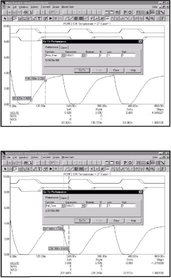
Figure 7-18 Measuring rise time

Figure 7-19 Measuring fall time

the difference between the X expression values, and places cursors at the two locations. The screen should look as shown at Figure 7-21.

31

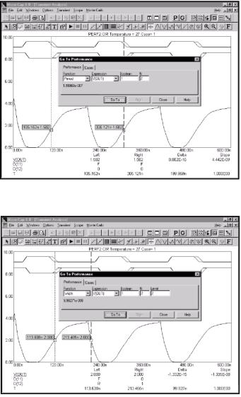
Figure 7-20 Measuring the pulse period

Figure 7-21 Measuring the pulse width

Select the X_Range function. Click on Go To. The screen looks like Figure 7-22.

32

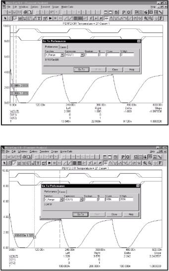
Figure 7-22 The X_Range function

Figure 7-23 The Y_Range function

X_Range locates the N'th instance of the YLow and YHigh values, places cursors at the data points and returns the difference between the X expression values. The Y_Range function works similarly.

33

Select it and set XLow = lOOn and XHigh = 200n, and click the Go To button. The result looks like Figure 7-23 (see above).

Figure 7-24 Measuring digital rise times

Figure 7-25 Measuring digital fall times

34

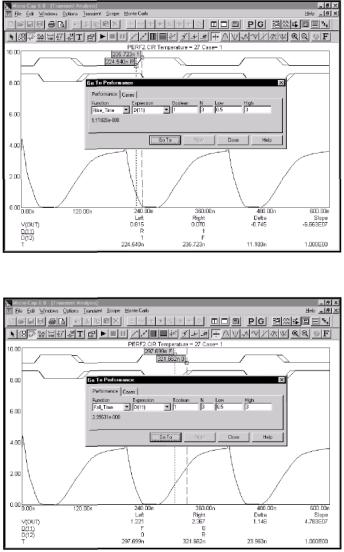
Performance functions also work on digital waveforms. Select D(l1) from the Expression list and Rise_Time from the Function list. Set N=2 and click the Go To button. The result looks like Figure 7-24.

Select the Fall_time function. The result for N=2 looks like Figure 7-25.

Animating an analysis

It is often useful to step through an analysis one time point at a time. Animation mode lets you do this and displays the node voltages and digital states on the schematic at each time point. To see how the mode works, load the file MIXED4. Select Transient from the Analysis menu. Press ALT + F4 to remove the Analysis

Limits dialog box. Click on the Tile Vertical button. Click on the Animate button, select the Wait for Key Press option, and

hit OK. Click on the Node Voltages Click on the Run button. Hold the Enter key down to observe each new data point being computed and printed on the schematic.

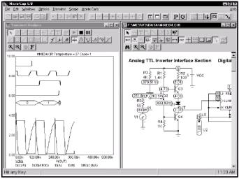
Figure 7-26 Animating an analysis

35

The figure above shows what the screen should look like midway through the run.

In this mode, MC6 computes a single data point, optionally prints the voltages/ states, currents, power, and conditions on the schematic, and then awaits a key press or time delay. It then repeats the cycle of compute, print, and pause until the run is complete. When Animate mode is canceled by clicking on the Don't Wait button in the Animate dialog box, the run continues in normal mode. To see both the schematic and analysis plot simultaneously, you must select either Tile Horizontal or Tile Vertical.

This option is available for AC, DC, and transient analysis, although it is most useful in the transient analysis of digital and mixed-mode circuits. Press ESC to stop the run, F3 to exit the analysis, and CTRL + F4 to close the file.

36

Задание 3

Прочтите и ответьте на вопросы.

1.Что позволяет моделировать модуль “Probe”?

2.Какие физические величины могут отображаться на графиках в ходе моделирования?

3.Можно ли наблюдать параллельно сигналы в разных точках схемы?

4.Как выбрать совокупность контрольных точек схемы?

5.Как от анализа по постоянной составляющей перейти к анализу по переменному току?

6.Каковы особенности проведения анализа при переменном токе?

What's in this chapter

Probe is an alternative tool for viewing the results of an analysis. It performs the selected analysis, saves the entire analysis in a disk file, then lets the user probe the schematic for waveforms or curves. Unlike a normal analysis, where only the waveforms specified in the Analysis Limits dialog box are saved, Probe saves everything, so you can decide what to plot after the analysis run. It is very much like probing a real circuit with an oscilloscope, spectrum analyzer, or curve tracer. In this chapter we demonstrate Probe's capabilities with several examples. The topics include:

•How Probe works

•Transient analysis variables

•Experimenting with Probe

•Navigating the schematic

•An AC example

•A DC example

37