

Linear Homogeneous Systems of de with variable coefficients
A normal linear system of differential equations with variable coefficients can be written as
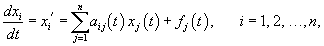
where xi (t) are unknown functions, which are continuous and differentiable on an interval [a, b]. The coefficients aij (t) and the free terms fi (t) are continuous functions on the interval [a, b]. Using vector-matrix notation, this system of equations can be written as
![]()
where
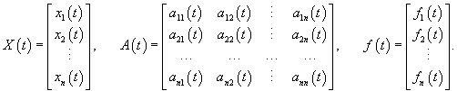
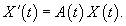
In the general case, the matrix A(t) and the vector functions X(t), f(t) can take both real and complex values. The corresponding homogeneous system with variable coefficients in vector form is given by
26) Fundamental System of Solutions and Fundamental Matrix
The vector functions x1(t), x2(t), ..., xn(t) are linearly dependent on the interval [a, b], if there are numbers c1, c2, ..., cn, not all zero, such that the following identity holds:
![]()
If this identity is satisfied only if
![]()
the vector functions xi (t) are called linearly independent on the given interval. Any system of n linearly independent solutions x1(t), x2(t), ..., xn(t) is called a fundamental system of solutions. A square matrix Φ(t) whose columns are formed by linearly independent solutions x1(t), x2(t), ..., xn(t) is called thefundamental matrix of the system of equations. It has the following form:
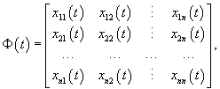
where xij (t) are the coordinates of the linearly independent vector solutions x1(t), x2(t), ..., xn(t). Note that the fundamental matrix Φ(t) is nonsingular, i.e. there always exists the inverse matrix Φ −1(t). Since the fundamental matrix has n linearly independent solutions, after its substitution into the homogeneous system we obtain the identity
![]()
We multiply this equation on the right by the inverse function Φ −1(t):
![]()
The resulting relation uniquely defines a homogeneous system of equations, given the fundamental matrix. The general solution of the homogeneous system is expressed in terms of the fundamental matrix in the form
![]()
where C is an n-dimensional vector consisting of arbitrary numbers. Let us mention an interesting special case of homogeneous systems. It turns out that if the product of the matrix A(t) and the integral of this matrix is commutative, i.e.
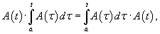
the fundamental matrix Φ(t) for such a system of equations is given by
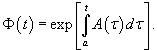
Such property is satisfied in the case of symmetric matrices and, in particular, in the case of diagonal matrices.
27. Wronskian and Liouville’s Formula.
W(t)=det
Theorem. If the system functions x 1, x 2, ..., x n are linearly dependent on the interval [a, b], then its Wronskian is identically to zero on this interval.
Theorem.
If x
1, x
2,
..., xn
– lenear
independent
system=>
W(t)≠0 , t [a,
b]
[a,
b]
Louville’s Formula.
Ly=0 (1)
W(x)=W( )
exp[-
)
exp[-
 (2)
(2)
Ly=
Proof:

 =
=
 +
+
 +
…+
+
…+ (все
матрицы в модуле)
(все
матрицы в модуле)
We put in (1) the last line
 =
=

 # LF
(луифид)
# LF
(луифид)
28. Method of Variation of Constants (Lagrange Method)
Now we consider the nonhomogeneous systems that can be written in the vector-matrix form as
![]()
The general solution of such a system is the sum of the general solution X0(t) of the corresponding homogeneous system and a particular solution X1(t) of the nonhomogeneous system, i.e.
![]()
where Φ(t) is a fundamental matrix, C is an arbitrary vector. The most common method for solving the nonhomogeneous systems is the method of variation of constants (Lagrange method). With this method, instead of the constant vector C, we consider the vector C(t) whose components are continuously differentiable functions of the independent variable t, i.e. we assume
![]()
Substituting this into the nonhomogeneous system, we find the unknown vector C(t):
![]()
Given that the matrix Φ(t) is nonsingular, we multiply this equation on the left by Φ−1(t):
![]()
After integration we obtain the vector C(t).