18. Reduction of order

case 1: DE of type

,

Example :

,

, , , .

case 2: DE of type

case 3: Homogeneous DE

Example:

case 4:

Example:

18. N-th Order Linear Homogeneous DE with Constant Coefficients:

19. Characteristic equation. The roots of the Characteristic Equation are Real and Multiple, Complex and Distinct, Complex and Multiple.

The linear homogeneous differential equation of the n-th order with constant coefficients can be written as

where a₁, a₂,..., a_n constants which may be real or complex. 

Let us consider in more detail the different cases of the roots of the characteristic equation and the corresponding formulas for the general solution of differential equations.

Case 1. All Roots of the Characteristic Equation are Real and Distinct

Assume that the characteristic equation L(λ) = 0 has n roots λ₁, λ₂,..., λ_n. In this case the general solution of the differential equation is written in a simple form:

where C₁, C₂,..., C_n are constants depending on initial conditions.

Case 2. The Roots of the Characteristic Equation are Real and Multiple

Let the characteristic equation L(λ) = 0 of degree n have m roots λ₁, λ₂,..., λ_m, the multiplicity of which, respectively, is equal to k₁, k₂,..., k_m. It is clear that the following condition is satisfied:

Then the general solution of the homogeneous differential equations with constant coefficients has the form

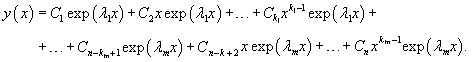
It is seen that the formula of the general solution has exactly k_i terms corresponding to each root λ_i of multiplicity k_i. These terms are formed by multiplying x to a certain degree by the exponential function exp(λ_i x). The degree of xvaries in the range from 0 to k_i − 1, where k_i is the multiplicity of the root λ_i.

Case 3. The Roots of the Characteristic Equation are Complex and Distinct

If the coefficients of the differential equation are real numbers, the complex roots of the characteristic equation will be presented in the form of conjugate pairs of complex numbers:

In this case the general solution is written as

Case 4. The Roots of the Characteristic Equation are Complex and Multiple

Here, each pair of complex conjugate roots α ± iβ of multiplicity k produces 2k particular solutions:

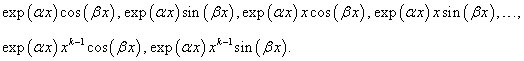
Then the part of the general solution of the differential equation corresponding to a given pair of complex conjugate roots is constructed as follows:

In general, when the characteristic equation has both real and complex roots of arbitrary multiplicity, the general solution is constructed as the sum of the above solutions of the form 1-4. 

18. N-th Order Linear Non-homogeneous DE with Constant Coefficients.

19. Method of Variation of Parameters

20. Method of Undetermined Coefficients

These equations have the form

where a₁, a₂,..., a_n are real or complex numbers, and the right-hand side f(x) is a continuous function on some interval [a, b].  Using the linear differential operator L(D) equal to

the nonhomogeneous differential equation can be written as

The general solution y(x) of the nonhomogeneous equation is the sum of the general solution y₀(x) of the correspondinghomogeneous equation and a particular solution y₁(x) of the nonhomogeneous equation:

For an arbitrary right side f(x), the general solution of the nonhomogeneous equation can be found using the method of variation of parameters. If the right-hand side is the product of a polynomial and exponential functions, it is more convenient to seek a particular solution by the method of undetermined coefficients.

Method of Variation of Parameters

Assume that the general solution of the homogeneous differential equation of the n-th order is known and given by

According to the method of variation of constants (or Lagrange method), we consider the functions C₁(x), C₂(x),...,C_n(x) instead of the regular numbers C₁, C₂,..., C_n. These functions are chosen so that the solution

satisfies the original nonhomogeneous equation.  The derivatives of n unknown functions C₁(x), C₂(x),..., C_n(x) are determined from the system of n equations:

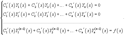
The determinant of this system is the Wronskian of Y₁, Y₂,..., Y_n forming a fundamental system of solutions. By the linear independence of these functions, the determinant is not zero and the system is uniquely solvable. The final expressions forthe functions C₁(x), C₂(x),..., C_n(x) can be found by integration.

Method of Undetermined Coefficients

If the right-hand side f(x) of the differential equation is a function of the form

where P_n(x), Q_m(x) are polynomials of degree n and m, respectively, then the method of undetermined coefficients may be used to find a particular solution.  In this case, we seek a particular solution in the form corresponding to the structure of the right-hand side of the equation. For example, if the function has the form

the particular solution is given by

where A_n(x) is a polynomial of the same degree n as P_n(x). The coefficients of the polynomial A_n(x) are determined by direct substitution of the trial solution y₁(x) in the nonhomogeneous differential equation.  In the so-called resonance case, when the number of α in the exponential function coincides with a root of the characteristic equation, an additional factor x^s, where s is the multiplicity of the root, appears in the particular solution.In the non-resonance case, we set s = 0.  The same algorithm is used when the right-hand side of the equation is given in the form

Here the particular solution has a similar structure and can be written as

where A_n(x), B_n(x) are polynomials of degree n (for n ≥ m), and the degree s in the additional factor x^s is equal tothe multiplicity of the complex root α ± βi in the resonance case (i.e. when the numbers α and β coincide with the complex root of the characteristic equation), and, accordingly, s = 0 in the non-resonance case.

Superposition Principle

The superposition principle is stated as follows. Let the right-hand side f(x) be the sum of two functions:

Suppose that y₁(x) is a solution of the equation

and the function y₂(x) is, accordingly, a solution of the second equation

Then the sum of the functions

will be a solution of the linear nonhomogeneous equation

Example:

Find the general solution of the differential equation  y''' + 3y'' − 10y' = x − 3. Solution.

First we find the general solution of the homogeneous equation

      

Calculate the roots of the characteristic equation:

      

      

      

The right side of the equation contains only a polynomial. However, if we take into account that exp(0) = 1, we see that in fact we have the resonance case (in disguised form) as one of the roots of the characteristic equation is also zero: λ₁ = 0. Therefore, we seek a particular solution in the form of

      

Substitute the derivatives

      

into the nonhomogeneous equation and determine the coefficients A, B:

      

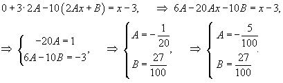
The particular solution y₁ is written as

      

Thus, the general solution of nonhomogeneous differential equation is given by