1. Differential equation of first order. Separable Equations

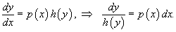
A first order differential equation y' = f(x,y) is called a separable equation if the function f(x,y) can be factored into the product of two functions of x and y:

where p(x) and h(y) are continuous functions.

Considering the derivative y' as the ratio of two differentials   we move dx to the right side and divide the equation by h(y):

Of course, we need to make sure that h(y) ≠ 0. If there's a number x₀ such that h(x₀) = 0, then this number will also be a solution of the differential equation. Division by h(y) causes loss of this solution.  Denoting  , we write the equation in the form

We have separated the variables so now we can integrate this equation:

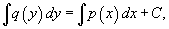
where C is an integration constant.  Calculating the integrals, we get the expression

representing the general solution of the separable differential equation.

Example:

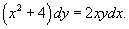
       1

      

      

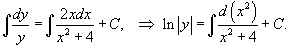
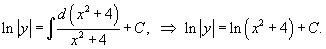
We can represent the constant C as lnC₁, where C₁ > 0. Then

      

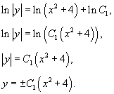
Thus, the given differential equation has the following solutions:

      

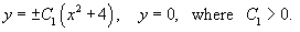
This answer can be simplified. Indeed, if using an arbitrary constant C, which takes values from −∞ to +∞, the solution can be written in the form:

      

When C = 0, it becomes y = 0. 

2. Homogeneous Equations. Linear de of first order.

A first order differential equation

is called homogeneous equation, if the right side satisfies the condition

for all t. In other words, the right side is a homogeneous function (with respect to the variables x and y) of the zero order:

Definition of Linear Equation of First Order

A differential equation of type

where a(x) and f(x) are continuous functions of x, is called a linear nonhomogeneous differential equation of first order.

We consider two methods of solving linear differential equations of first order:

• Using an integrating factor;

• Method of variation of a constant.

Using an Integrating Factor

If a linear differential equation is written in the standard form:

the integrating factor is defined by the formula

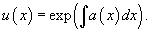
Multiplying the left side of the equation by the integrating factor u(x) converts the left side into the derivative of the producty(x)u(x).  The general solution of the differential equation is expressed as follows:

where C is an arbitrary constant.

Method of Variation of a Constant

This method is similar to the previous approach. First it's necessary to find the general solution of the homogeneous equation:

The general solution of the homogeneous equation contains a constant of integration C. We replace the constant C with a certain (still unknown) function C(x). By substituting this solution into the nonhomogeneous differential equation, we can determine the function C(x).  The described algorithm is called the method of variation of a constant. Of course, both methods lead to the same solution.