Код программы Matlab

%display spectors

sp = fft(x1); % spector x1

figure(11);

plot(abs(sp));

sp = fft(x2); % spector x2

figure(12);

plot(abs(sp));

sp = fft(x3); % spector x3

figure(13);

plot(abs(sp));

sp = fft(x4); % spector x4

figure(18);

plot(abs(sp));

sp = fft(x5); % spector x5

figure(20);

plot(abs(sp));

%autocorrelation

figure(21);

[r, lags] = xcorr(x1, 'coeff');

plot(lags, r, 'r'); grid on;

figure(22);

[r, lags] = xcorr(x2, 'coeff');

plot(lags, r, 'b'); grid on;

figure(23);

[r, lags] = xcorr(x3, 'coeff');

plot(lags, r, 'g'); grid on;

figure(24);

[r, lags] = xcorr(x4, 'coeff');

plot(lags, r, 'r'); grid on;

figure(25);

[r, lags] = xcorr(x5, 'coeff');

plot(lags, r, 'r'); grid on;

%FT from spectors

figure(26);

[r, lags] = xcorr(x1, 'coeff');

plot(lags, fft(r), 'r'); grid on;

figure(27);

[r, lags] = xcorr(x2, 'coeff');

plot(lags, fft(r), 'b'); grid on;

figure(28);

[r, lags] = xcorr(x3, 'coeff');

plot(lags, fft(r), 'g'); grid on;

figure(29);

[r, lags] = xcorr(x4, 'coeff');

plot(lags, fft(r), 'r'); grid on;

figure(30);

[r, lags] = xcorr(x5, 'coeff');

plot(lags, fft(r), 'r'); grid on;

Пункт 3

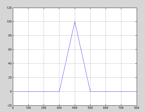
Рис 28. КФ сигнала без шума

Отношение С/Ш: 39.1320

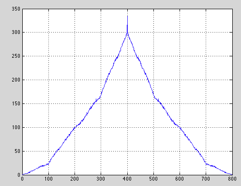
Рис 29. КФ сигнала с шумом

Отношение С/Ш: 27.0028

Код программы Matlab

%--aircrft height --%

figure(69);

s1 = [ones(1,100) zeros(1,100)];

s2 = [zeros(1,200) s1]; %shifted signal

noise = rand(1,length(s1));

x = 20*log(10*(s1/noise)); %rate of signal/noise

disp(x);

x1 = xcorr(s2); %autocorrelation of shifted signal

plot(1:length(x1), x1);

grid on;

figure(70);

noise = rand(1,length(s2));

x = 20*log(10*(s2/noise)); %rate of signal/noise

disp(x);

x1 = xcorr(s2+noise); %correlation of shifted signal

plot(1:length(x1), x1);

grid on;

Вывод

В ходе данной лабораторной работы мы исследовали построение КФ и АКФ, изучили построение спектров и преобразования Фурье в среде matlab, исследовали зависимость σ, σ2 от выбора интервала осреднения.