Laboratory Work 13 approximation done by the least-squares method

Purpose of work: to learn to describe table functions by analytical expressions.

13.1 Theoretical Data

Approximation ( Lain : approximare – to approach) – approximate expression of some values through other, simpler ones.

Table function approximation

y_i = f(x_i) , (13.1)

i=1,2,…,n . (13.2)

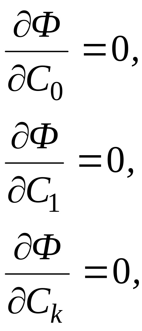
made by the least-squares method consists in determining some analytical F(x),function parametres that provide the functional minimization.

(13.3)

If the stepped polynomial

(13.4)

is chosen to be the approximating function, the task consists in determining the vector of the coefficients by solving the system oflinear equations of (k+1) order.

(13.5)

Where (13.6)

(13.7)

m=0,1,…,k.. (13.8)

After the transformations the system (13.5) is of the form :

(13.9)

The system (13.9) shows that the the elements of the matrix of the coefficients A and the vectors of the free terms can be described by the formulae:

(13.10)

When the coefficients are determined, the system (13.9) can be solved by any of the known methods, for example Gaussian.

Approximation done by the least-squares method is often used to smooth the table functions obtained as a result of the experiment as well as to reduce the amount of information on the table functions when the requirements on computation accuracy are not strict..

13.2 Task

Approximate the table function given in the table of the work 12 by the step polynomial of the k order by the leat-squares method. For odd variants k=3, for even ones - k=2. Illustrate the results by graphs. Do the programme twice with different number of the table points (n=9 і n=5). Evaluate theinfluence of the number oа points on the approximation accuracy.

13.3 Methodical Recommendations

When standard programmes are applied to solve the equation system (13.9) the indices of the standard equation system ( which don’t have coefficients with zero indices) are coordinated with those of the system (13.9). The coordination consists in change of the formulae ( 13.10).

Laboratory Work 14 numerical integration

Purpose of work: to learn to compute integrals from the functions given in the table and analytical ways.

14.1 Theoretical Data

Tasks to compute integrals appear practically in all spheres of applied mathematics.

The basics of the numerivcal integration methods consists in the fact that the interval [a, b] is split into sections on which the curve described by the sub-integral fucntion f(x), is replaced by some other curve for which theintegral computing is done by rather simple formulae, and then all squares are summed.

When interpolating polymomials replace the sub-integral function the so called quadrature formula is obtained. The quadrature formulae for th einterpolation equidistance nodes are called the formulae of Newton- Cotes.

Depending on the degree of the interpolating polinomial we distinguish the methods of rectangles, trapezium and quadratic trapezium, or Symson method.

The main formulae and indices which charaterise these methods when the integration interval is divided into equal sections are given in the table 14.1, where the following symbols are accepted:

n – the number of the layout sections,

- integration step

(14.1)

The method mistake is detrmined by the value of the integral of the interpolation polynomial remainder term. In the formulae to evaluate the mistake M_i the maximum value of the i derivative on the interval [a, b].

Table 14.1 Task for the Laboratory Work №14

Name of the method	Interpolating polynomial degree		Mistake
Rectangle	0
Trapezium	1
Simpson	2

When Simson method is applied the number of the layout sections is even (n=2k) and all the sections are identical. Under the irregular integration interval layout the rectangle and trapezium methods are applied. For them the numerical integration formulae are of the form:

(14.2)

According to the rectangle method,

(14.3)

According to the trapezium method

To provide the required integration accurcay the algorithms with the step automated choiceare used. The integral value computing is done by one of the examined methods with the initial step h, and then these computations are repaetaed with the half-step . If it appears that

(14.4)

Where - the integration permissible mistake

The computing is stopped, if not the further step split is done.

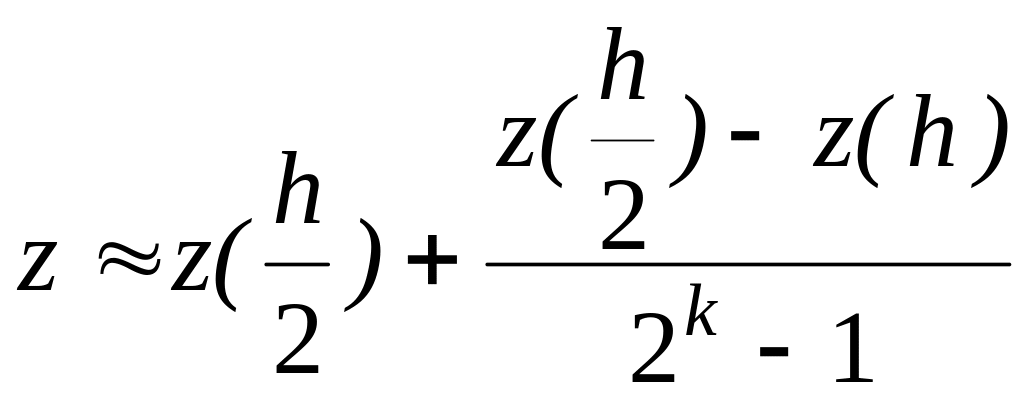
The integral approximate value obtained by this method can be specified by the extrapolation transition to the limit proposed by Richardson:

, (14.5)

1 – for the rectanle method ,

Where k= 2 – for the trapezium method,

3 –or the Sipson method .

14.2 Task

14.2.1 Table Function Integration

Compute the integral from the table function given in the table 14.2. Odd variants use the trapezium method under the interval irregular layout of integration and the method of Simpson under the regular one. The even varinats use the rectangle method and that of trapezium in analogous cases.

14.2.2 Integration of the Functions Given Analitically

Compute theintended integral

For the function given in the table 14.2 on the intended interval [a,b] with the intended accuracy ,using the step automated choice method specified in the table

14.3 Methodical Recommendations

To have the result visual verification build the sub-integration function graph and place it on the line parallel to the abscissa axis on the level of

If the solution is correct the square limited by the sub-integral curve and lines х=а, x=b і y=0, equals to the square of the rectangle limited by the line sections y=y_сp , x=a, x=b, y=0.

Tabel 14.2 Output Data for the Laboratory Work №14

Variants	Method		f(x)	a	b	Parametres
1	2	3	4	5	6	7
1	Rectangle	10-5		0		=0,182
2	Sipmson	10-3
3	Trapezium	10-4		0		c=0,953 d=2,295
4	Rectangle	10-2
5	Trapezium	10-6		0	1	c=3,18 d=-1,37
6	Simpson	10-3
7	Rectangle	10-2		0		m=3
8	Trapezium	10-4
9	The same	10-5		0	1	c=1,21
10	Simpson	10-3
11	Trapezium	10-2		0		c=8,53 d=0,524
12	Rectangle	10-4
13	Simpson	10-5		0	1	c=0,732
14	Trapezium	10-3
Continuation of the table 14.2
1	2	3	4	5	6	7
15	Rectangle	10-4		0		c=3,76 d=8,39
16	Trapezium	10-2
17	Simpson	10-6		0	1	c=4,18
18	Trapezium	10-3
19	The same	10-2		0	1	c=0,874
20	Rectangle	10-4
21	Simpson	10-5		1	2	c=2
22	Trapezium	10-3
23	Rectangle	10-2		1	5
24	Simpson	10-4
25	The same	10-5		0		c=0,5
26	Trapezium	10-3