18

Subject “ AERO-HYDRO-GAS DYNAMICS

”MODULUS TEST WORK № 2 PROBLEMS

Problems of the first level

1. Ratio between a vortex strength and velocity circulation around of it.

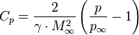
2. Give a definition of a coefficient of pressure

The pressure coefficient is a dimensionless number which describes the relative pressures throughout a flow field in fluid dynamics. The pressure coefficient is used in aerodynamics andhydrodynamics. Every point in a fluid flow field has its own unique pressure coefficient,  .

In many situations in aerodynamics and hydrodynamics, the pressure coefficient at a point near a body is independent of body size. Consequently an engineering model can be tested in a wind tunnel or water tunnel, pressure coefficients can be determined at critical locations around the model, and these pressure coefficients can be used with confidence to predict the fluid pressure at those critical locations around a full-size aircraft or boat.

The pressure coefficient is a parameter for studying the flow of incompressible fluids such as water, and also the low-speed flow of compressible fluids such as air. The relationship between the dimensionless coefficient and the dimensional numbers is ^[1]

^[2]

where:

 is the pressure at the point at which pressure coefficient is being evaluated

 is the pressure in the freestream (i.e. remote from any disturbance)

 is the freestream fluid density (Air at sea level and 15 °C is 1.225  )

 is the freestream velocity of the fluid, or the velocity of the body through the fluid

Using Bernoulli's Equation, the pressure coefficient can be further simplified for incompressible, lossless, and steady flow:^[3]

where V is the velocity of the fluid at the point at which pressure coefficient is being evaluated.

This relationship is also valid for the flow of compressible fluids where variations in speed and pressure are sufficiently small that variations in fluid density can be ignored. This is a reasonable assumption when the Mach Number is less than about 0.3.

•  of zero indicates the pressure is the same as the free stream pressure.

 of one indicates the pressure is stagnation pressure and the point is a stagnation point.

 of minus one is significant in the design of gliders because this indicates a perfect location for a "Total energy" port for supply of signal pressure to the Variometer, a special Vertical Speed Indicator which reacts to vertical movements of the atmosphere but does not react to vertical maneuvering of the glider.

In the fluid flow field around a body there will be points having positive pressure coefficients up to one, and negative pressure coefficients including coefficients less than minus one, but nowhere will the coefficient exceed plus one because the highest pressure that can be achieved is the stagnation pressure. The only time the coefficient will exceed plus one is when advanced boundary layer control techniques, such as blowing, is used.

Compressible flow [edit]

In the flow of compressible fluids such as air, and particularly the high-speed flow of compressible fluids,   (the dynamic pressure) is no longer an accurate measure of the difference between stagnation pressure and static pressure. Also, the familiar relationship that stagnation pressure is equal to total pressure does not always hold true. (It is always true in isentropic flow but the presence of shock waves can cause the flow to depart from isentropic.) As a result, pressure coefficients can be greater than one in compressible flow.^[4]

 greater than one indicates the freestream flow is compressible.

Pressure distribution [edit]

An airfoil at a given angle of attack will have what is called a pressure distribution. This pressure distribution is simply the pressure at all points around an airfoil. Typically, graphs of these distributions are drawn so that negative numbers are higher on the graph, as the   for the upper surface of the airfoil will usually be farther below zero and will hence be the top line on the graph.

 and   relationship [edit]

The coefficient of lift for an airfoil with strictly horizontal surfaces can be calculated from the coefficient of pressure distribution by integration, or calculating the area between the lines on the distribution. This expression is not suitable for direct numeric integration using the panel method of lift approximation, as it does not take into account the direction of pressure-induced lift.

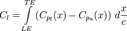
where:

 is pressure coefficient on the lower surface

 is pressure coefficient on the upper surface

 is the leading edge

 is the trailing edge

When the lower surface   is higher (more negative) on the distribution it counts as a negative area as this will be producing down force rather than lift.

3. Write Zhukovsky formula for a lift, to term values, which are contained in this formula.

The Kutta–Joukowski theorem is a fundamental theorem of aerodynamics. It is named after the German Martin Wilhelm Kutta and the Russian Nikolai Zhukovsky (or Joukowski) who first developed its key ideas in the early 20th century. The theorem relates the lift generated by a right cylinder to the speed of the cylinder through the fluid, the density of the fluid, and the circulation. The circulation is defined as the line integral, around a closed loop enclosing the cylinder or airfoil, of the component of the velocity of the fluid tangent to the loop.^[1] The magnitude and direction of the fluid velocity change along the path.

The flow of air in response to the presence of the airfoil can be treated as the superposition of a translational flow and a rotational flow. It is, however, incorrect to think that there is a vortex like atornado encircling the cylinder or the wing of an airplane in flight. It is the integral's path that encircles the cylinder, not a vortex of air. (In descriptions of the Kutta–Joukowski theorem the airfoil is usually considered to be a circular cylinder or some other Joukowski airfoil.)

The theorem refers to two-dimensional flow around a cylinder (or a cylinder of infinite span) and determines the lift generated by one unit of span. When the circulation   is known, the lift   per unit span (or  ) of the cylinder can be calculated using the following equation:^[2]

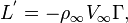
(1)

where   and   are the fluid density and the fluid velocity far upstream of the cylinder, and   is the (anticlockwise positive) circulation defined as the line integral,

around a closed contour   enclosing the cylinder or airfoil and followed in the positive (anticlockwise) direction. This path must be in a region of potential flow and not in the boundary layer of the cylinder. The integrand   is the component of the local fluid velocity in the direction tangent to the curve   and   is an infinitesimal length on the curve,  . Equation (1) is a form of theKutta–Joukowski theorem.

Kuethe and Schetzer state the Kutta–Joukowski theorem as follows:^[3]

The force per unit length acting on a right cylinder of any cross section whatsoever is equal to  , and is perpendicular to the direction of 

4. Give the definition of a shock wave, to term conditions, at which there is a shock wave.

A shock wave is a type of propagating disturbance. Like an ordinary wave, it carries energy and can propagate through a medium (solid, liquid, gas orplasma) or in some cases in the absence of a material medium, through a field such as the electromagnetic field. Shock waves are characterized by an abrupt, nearly discontinuous change in the characteristics of the medium.^[1] Across a shock there is always an extremely rapid rise in pressure,temperature and density of the flow. In supersonic flows, expansion is achieved through an expansion fan. A shock wave travels through most media at a higher speed than an ordinary wave.

Shock waves can be:

• Normal: at 90° (perpendicular) to the shock medium's flow direction.

• Oblique: at an angle to the direction of flow.

• Bow: Occurs upstream of the front (bow) of a blunt object when the upstream velocity exceeds Mach 1.

Some other terms

• Shock Front: an alternative name for the shock wave itself

• Contact Front: in a shock wave caused by a driver gas (for example the "impact" of a high explosive on the surrounding air), the boundary between the driver (explosive products) and the driven (air) gases. The Contact Front trails the Shock Front.

5. Two types of boundary layers (with respect to a regime of flow).

 A boundary layer is the layer of fluid in the immediate vicinity of a bounding surface where the effects of viscosity are significant. In the Earth's atmosphere, the planetary boundary layer is the air layer near the ground affected by diurnal heat, moisture or momentum transfer to or from the surface. On an aircraft wing the boundary layer is the part of the flow close to the wing, where viscous forces distort the surrounding non-viscous flow. See Reynolds number.

Boundary layer visualization, showing transition from laminar to turbulent condition

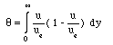
6. Give a definition of a boundary layer thickness.

The boundary layer thickness, δ, is defined as the distance required for the flow to nearly reach U_e. We might take an arbitrary number (say 99%) to define what we mean by "nearly", but certain other definitions are used most frequently. The displacement thickness and momentum thickness are alternative measures of boundary layer thickness and are used in the calculation of various boundary layer properties. The displacement thickness is defined by considering the total mass flow through the boundary layer. This mass flow is the same as if the boundary layer were completely at rest, with a thickness, δ*: 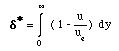For laminar boundary layers δ* is about one third of the distance to the edge of the boundary layer, δ. The momentum thickness, θ, is defined similarly, using the momentum flux rather than the mass flux: For laminar boundary layers, δ tends to be about an order of magnitude greater than θ. The ratio of δ* to θ is termed the shape factor, H:

7. Two types of boundary layers (with respect to a regime of flow).

A boundary layer may be laminar or turbulent. A laminar boundary layer is one where the flow takes place in layers, i.e., each layer slides past the adjacent layers. This is in contrast to Turbulent Boundary Layers shown in Fig.6.2 where there is an intense agitation.

In a laminar boundary layer any exchange of mass or momentum takes place only between adjacent layers on a microscopic scale which is not visible to the eye. Consequently molecular viscosity   is able predict the shear stress associated. Laminar boundary layers are found only when the Reynolds numbers are small.

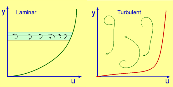
Figure 6.2: Typical velocity profiles for laminar and turbulent boundary layers

A turbulent boundary layer on the other hand is marked by mixing across several layers of it. The mixing is now on a macroscopic scale. Packets of fluid may be seen moving across. Thus there is an exchange of mass, momentum and energy on a much bigger scale compared to a laminar boundary layer. A turbulent boundary layer forms only at larger Reynolds numbers. The scale of mixing cannot be handled by molecular viscosity alone. Those calculating turbulent flow rely on what is called Turbulence Viscosity or Eddy Viscosity, which has no exact expression. It has to be modelled. Several models have been developed for the purpose.

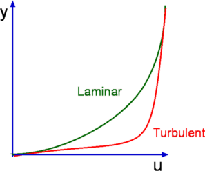
Figure 6.3: Typical velocity profiles for laminar and turbulent boundary layers

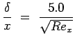
As a consequence of intense mixing a turbulent boundary layer has a steep gradient of velocity at the wall and therefore a large shear stress. In addition heat transfer rates are also high. Typical laminar and turbulent boundary layer profiles are shown in fig.6.3. Typical velocity profiles for laminar and turbulent boundary layers Growth Rate (the rate at which the boundary layer thickness   of a laminar boundary layer is small. For a flat plate it is given by

(6.1)

where Re_x is the Reynolds Number based on the length of the plate. For a turbulent flow it is given by

(6.2)

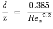
Wall shear stress is another parameter of interest in boundary layers. It is usually expressed as Skin friction defined as

(6.3)

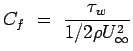
where   is the wall shear stress given by

(6.4)

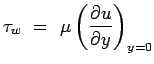
and   is the free stream speed.

Skin friction for laminar and turbulent flows are given by

	, Laminar
	,Turbulent

Boundary layer equations 

The deduction of the boundary layer equations was one of the most important advances in fluid dynamics (Anderson, 2005). Using an order of magnitude analysis, the well-known governingNavier–Stokes equations of viscous fluid flow can be greatly simplified within the boundary layer. Notably, the characteristic of the partial differential equations (PDE) becomes parabolic, rather than the elliptical form of the full Navier–Stokes equations. This greatly simplifies the solution of the equations. By making the boundary layer approximation, the flow is divided into an inviscid portion (which is easy to solve by a number of methods) and the boundary layer, which is governed by an easier to solve PDE. The continuity and Navier–Stokes equations for a two-dimensional steady incompressible flow in Cartesian coordinates are given by

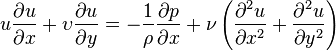
where   and   are the velocity components,   is the density,   is the pressure, and   is the kinematic viscosity of the fluid at a point.

The approximation states that, for a sufficiently high Reynolds number the flow over a surface can be divided into an outer region of inviscid flow unaffected by viscosity (the majority of the flow), and a region close to the surface where viscosity is important (the boundary layer). Let   and   be streamwise and transverse (wall normal) velocities respectively inside the boundary layer. Using scale analysis, it can be shown that the above equations of motion reduce within the boundary layer to become

and if the fluid is incompressible (as liquids are under standard conditions):

The asymptotic analysis also shows that  , the wall normal velocity, is small compared with   the streamwise velocity, and that variations in properties in the streamwise direction are generally much lower than those in the wall normal direction.

Since the static pressure   is independent of  , then pressure at the edge of the boundary layer is the pressure throughout the boundary layer at a given streamwise position. The external pressure may be obtained through an application of Bernoulli's equation. Let   be the fluid velocity outside the boundary layer, where   and   are both parallel. This gives upon substituting for   the following result

with the boundary condition

For a flow in which the static pressure   also does not change in the direction of the flow then

so   remains constant.

Therefore, the equation of motion simplifies to become

These approximations are used in a variety of practical flow problems of scientific and engineering interest. The above analysis is for any instantaneous laminar or turbulent boundary layer, but is used mainly in laminar flow studies since the mean flow is also the instantaneous flow because there are no velocity fluctuations present.

Turbulent boundary layers [edit]

The treatment of turbulent boundary layers is far more difficult due to the time-dependent variation of the flow properties. One of the most widely used techniques in which turbulent flows are tackled is to apply Reynolds decomposition. Here the instantaneous flow properties are decomposed into a mean and fluctuating component. Applying this technique to the boundary layer equations gives the full turbulent boundary layer equations not often given in literature:

Using the same order-of-magnitude analysis as for the instantaneous equations, these turbulent boundary layer equations generally reduce to become in their classical form:

The additional term   in the turbulent boundary layer equations is known as the Reynolds shear stress and is unknown a priori. The solution of the turbulent boundary layer equations therefore necessitates the use of a turbulence model, which aims to express the Reynolds shear stress in terms of known flow variables or derivatives. The lack of accuracy and generality of such models is a major obstacle in the successful prediction of turbulent flow properties in modern fluid dynamics.

A laminar sub-layer exists in the turbulent zone; it occurs due to those fluid molecules which are still in the very proximity of the surface, where the shear stress is maximum and the velocity of fluid molecules is zero.

8. Draw approximately the charts of change of speed along a normal to a surface accordingly in laminar and turbulent boundary layers.

9. Give a definition of a mixed boundary layer.

10. Give a definition of a transition point in a boundary layer.

11. In what boundary layer of a type the stress of friction on a surface is more?

12. Give a definition of a critical Reynold's number in a boundary layer, ratio between a critical Reynold's number and transition point.

13. Explain a phenomenon of boundary layer separation. What condition is necessarily executed in a separation point of a boundary layer?

14. The purpose of control of a boundary layer.

15. To term ways of boundary layer control.

16. Give a definition of total aerodynamic force.

17. Give the definitions of lift force, drag force, lateral force.

A fluid flowing past the surface of a body exerts surface force on it. Lift is the component of this force that is perpendicular to the oncoming flow direction.^[1] It contrasts with the drag force, which is the component of the surface force parallel to the flow direction. If the fluid is air, the force is called an aerodynamic force.

If the lift coefficient for a wing at a specified angle of attack is known (or estimated using a method such as thin airfoil theory), then the lift produced for specific flow conditions can be determined using the following equation:^[89]

where

L is lift force,

• ρ is air density

• v is true airspeed,

• A is planform area, and

•  is the lift coefficient at the desired angle of attack, Mach number, and Reynolds number^[90]

In aerodynamics, aerodynamic drag is the fluid drag force that acts on any moving solid body in the direction of the fluid freestream flow.^[1] From the body's perspective (near-field approach), the drag comes from forces due to pressure distributions over the body surface, symbolized  , and forces due to skin friction, which is a result of viscosity, denoted  . Alternatively, calculated from the flowfield perspective (far-field approach), the drag force comes from three natural phenomena: shock waves, vortex sheet, and viscosity..

18. Give the definitions of aerodynamic pitching moments, rolling, yawing.

In aerodynamics, the pitching moment on an airfoil is the moment (or torque) produced by the aerodynamic force on the airfoil if that aerodynamic force is considered to be applied, not at the center of pressure, but at the aerodynamic center of the airfoil. The pitching moment on the wing of an airplane is part of the total moment that must be balanced using the lift on the horizontal stabilizer.^[1]