Iminfo('filename')

The information can be stored as a structure variable from which values can be retrieved:

pinfo = iminfo('filename');

pinfo.Width

2. Creating the Negative of an Image

In order to see the negative of the image, you will need to change the values in the image

matrix to double precision. This is done to invert the color matrix. The code below

negates the image:

Myimage = imread('exper.jpg');

negImage = double(Myimage); % Convert the image matrix to double

negImageScale = 1.0/max(negImage(:)); % Find the max value in this

% new array and take its

% inverse

negImage = 1 - negImage*negImageScale; % Multiply the double image

% matrix by the factor of

% negImageScale and subtract

% the total from 1

figure; % Draw the figure

imshow(negImage); % Show the new image

The above manipulations will result in a negative image that is exactly opposite in color to the original image.

3. Rgb Components of an Image

MatLab has the ability to find out exactly how much Red, Green, Blue content there is in

an image. You can find this out by selecting only one color at a time and viewing the

image in that color. The following code allows you to view the Red content of an image:

redimage = Myimage; % Create a new matrix equal to the matrix

% of your original image.

redimage (:, :, 2:3) = 0; % This selectively nullifies the second

% and third columns of the colormap

% matrix which are part of the original matrix. Since the colors

% are mapped using RGB, or columns with values of Red, Green and

% Blue, so we can selectively nullify the green and blue columns to

% obtain only the red part of the image.

imshow(redimage); % show the redimage that you just created.

Similarly, we can do the same with the green and blue components of the image. Just

keep in mind the format of the array

Red : Green : Blue

1 2 3

Try checking the blue component of the image. The only thing you will need to change is

the column numbers at the end of the statement.

blueimage = Myimage; % Create a new matrix equal to the matrix

% of your original image.

blueimage(:, :, 1:2) = 0; % Note the difference in column

% numbers.

imshow(blueimage); % Display the blueimage you just created.

Now try the green component yourself. There is a little trick to this.

After trying the green component of the image, try to see two components at a time. You

can do this by nullifying only one column at a time instead of two. (Hint: You only need

to put one number instead of 1:2 or 1:2:3 etc. Just write 1 or 2 or 3 to see the

combinations and note them.)

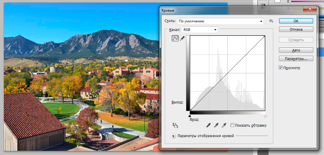
4. Gamma Scaling of an Image

Gamma scaling is an important concept in graphics and games. It relates to the pixel

intensities of the image. The format is simple:

J = imadjust(I, [low high], [bottom top], gamma);

This transforms the values in the intensity image I to values in J by mapping values

between low and high to values between bottom and top. Values below low and above

high are clipped. That is, values below low map to bottom, and those above high map to

top. You can use an empty matrix ([]) for [low high] or for [bottom top] to specify the

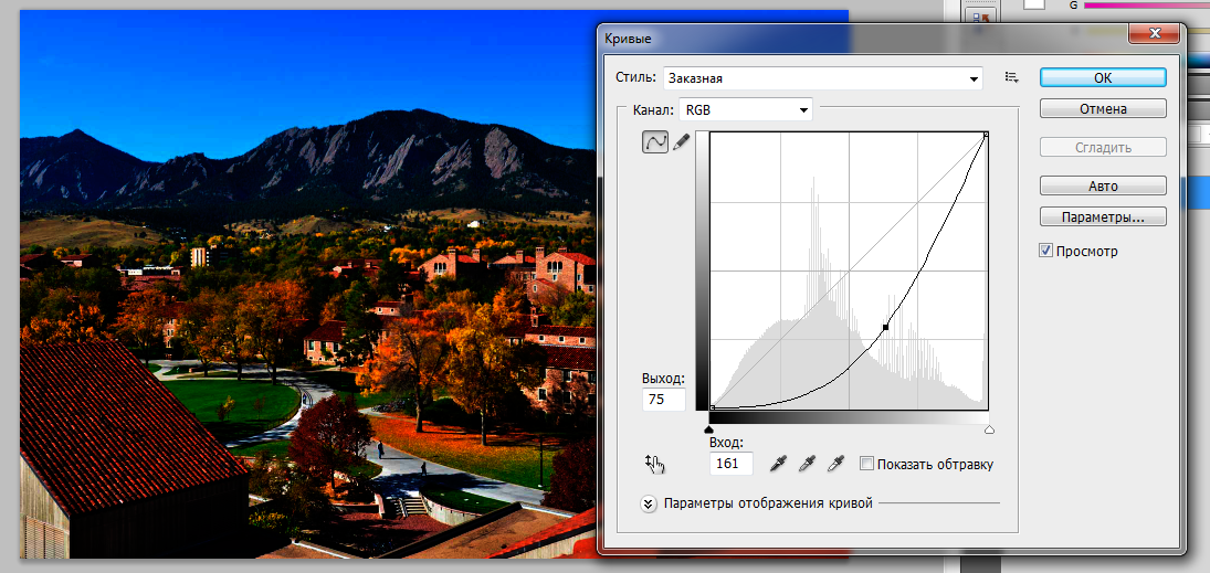
default of [0 1]. The variable gamma specifies the shape of the curve describing the

relationship between the values in I and J. If gamma is less than 1, the mapping is

weighted toward higher (brighter) output values. If gamma is greater than 1, the mapping

is weighted toward lower (darker) output values. If you omit the argument, gamma

defaults to 1 (linear mapping). Now try the following gamma variations and note down

the changes in intensities of the image.

NewImage = imadjust(Myimage, [.2, .7], []);

figure;

imshow(NewImage);

Note that the original image has gamma at default since there is no value of gamma

added. Now try this:

NewImage = imadjust(Myimage, [.2, .7], [], .2);

figure;

imshow(NewImage);

Note the difference? The gamma has been changed, so we see a change in the image

intensity. The intensity of each pixel in the image has increased. This clarifies the

explanation of gamma above. Now try a new value of gamma. This time use a value of 2

instead of .2.

Newimage = imadjust(x, [.2, .7], [], 2);

figure;

imshow(Newimage);

What happened? How did this change affect the gamma? Comment on your findings.

Тоновые кривые (Ctrl+M)