

1_c034481
.pdfDownloaded by 94.180.100.60 on November 25, 2018 | http://arc.aiaa.org | DOI: 10.2514/1.C034481
JOURNAL OF AIRCRAFT
Vol. 55, No. 4, July–August 2018
Sixth Drag Prediction Workshop Results Using FUN3D with k-kL-MEAH2015 Turbulence Model
K. S. Abdol-Hamid, Jan-Reneé Carlson,† Christopher L. Rumsey,‡ Elizabeth M. Lee-Rausch,§ and
Michael A. Park†
NASA Langley Research Center, Hampton, Virginia 23681
DOI: 10.2514/1.C034481
The Common Research Model wing/body configuration is investigated with the k-kL-MEAH2015 turbulence model implemented in FUN3D. This includes results presented at the Sixth Drag Prediction Workshop and additional results generated after the workshop with a nonlinear quadratic constitutive relation variant of the same turbulence model. The workshop-provided grids are used, and a uniform grid refinement study is performed at the design condition. A large variation between results with and without a reconstruction limiter is exhibited on “medium” grid sizes, indicating that the medium grid size is too coarse for drawing conclusions in comparison with experiment. This variation is reduced with grid refinement. At a fixed angle of attack near design conditions, the quadratic constitutive relation variant yielded decreased lift and drag compared with the linear eddy-viscosity model by an amount that was approximately constant with grid refinement. The k-kL-MEAH2015 turbulence model produced wing–root junction flow behavior consistent with wind-tunnel observations.
|
|
Nomenclature |
bref |
= |
wing semispan |
CD |
= |
drag coefficient |
Cfx |
= x component of skin friction coefficient |
|
CL |
= |
lift coefficient |
Cm |
= |
pitching moment coefficient |
Cp |
= |
surface pressure coefficient |
c |
= |
local chord |
cref |
= |
mean aerodynamic chord |
h |
= |
characteristic grid spacing |
M∞ |
= |
freestream Mach number |
N |
= number of nodes in grid |
|
Re |
= |
Reynolds number |
Sref |
= |
half-wing reference area |
α= angle of attack, deg
η= wingspan location
I.Introduction
THE AIAA Applied Aerodynamics Technical Committee conducted their sixth Drag Prediction Workshop (DPW-VI)¶ in the summer of 2016 to continue the evaluation of computational
fluid dynamics (CFD) transonic cruise drag predictions for subsonic transports. The stated objectives of the workshop were as follows: 1) to build on the success of the past five AIAA Drag Prediction Workshops (DPW-I–V), 2) to assess the state-of-the-art computational methods as practical aerodynamic tools for aircraft force and moment prediction of industry-relevant geometries, 3) to provide an
Presented as Paper 2017-0962 at the 55th AIAA Aerospace Sciences Meeting, Grapevine, TX, 9–13 January 2017; received 23 March 2017; revision received 31 May 2017; accepted for publication 14 June 2017; published online Open Access 18 July 2017. This material is declared a work of the U.S. Government and is not subject to copyright protection in the United States. All requests for copying and permission to reprint should be submitted to CCC at www.copyright.com; employ the ISSN 0021-8669 (print) or 15333868 (online) to initiate your request. See also AIAA Rights and Permissions www.aiaa.org/randp.
*Senior Research Scientist, Configuration Aerodynamics Branch, Mail Stop 499. Associate Fellow AIAA.
†Research Scientist, Computational AeroSciences Branch, Mail Stop 128. Senior Member AIAA.
‡Senior Research Scientist, Computational AeroSciences Branch, Mail Stop 128. Fellow AIAA.
§Assistant Branch Head, Computational AeroSciences Branch, Mail Stop 128. Associate Fellow AIAA.
¶Data available online at https://aiaa-dpw.larc.nasa.gov [retrieved 12 September 2016].
impartial forum for evaluating the effectiveness of existing computer codes and modeling techniques using Navier–Stokes solvers, and 4) to identify areas needing additional research and development. The focus of this workshop was the NASA Common Research Model (CRM) with wind-tunnel measured wing twist; both wing/body (WB) and wing/body/nacelle/pylon configurations were considered. CFD predictions of absolute and incremental force and moment values were examined and compared. The workshop included grid convergence and code verification studies as well as an angle-of- attack sweep with static aeroelastic deformations. As with prior workshops, grids were made available for all required cases.
Results for the DPW-VI required case studies were submitted to the workshop for the FUN3D [1–4] unstructured-grid Reynolds-averaged Navier–Stokes (RANS) solver on a set of workshop-supplied nodebased mixed-element meshes. FUN3D has been used in previous workshop studies, including DPW-IV [5] and DPW-V [6]. The prior FUN3D workshop studies focused on the use of the standard Spalart– Allmaras (SA) turbulence model. For the DPW-IV grid convergence study at the design lift condition, FUN3D total force/moment predictions with the SA model were within one standard deviation of the workshop core solution medians. The DPW-IV downwash study and Reynolds number study results also compared well with the range of results shown in the workshop presentations. Similarly, the FUN3D results from the DPW-V grid convergence study compared closely with results from other codes when using the SA model. However, results from the DPW-V buffet study produced a larger variation than the design case primarily due to the large differences in the predicted side-of-body separation. Park et al. [6] summarize the DPW-IV methods and size of the simulated side-of-body separations. They also studied the impact of modeling differences and grid effects on separation extent in the context of DPW-V. A large wing–root separation bubble was not observed in the wind-tunnel tests.
FUN3D results for DPW-VI were submitted for the SA turbulence model and for a recently developed k-kL-MEAH2015 turbulence model [7]. The k-kL-MEAH2015 model has been implemented in FUN3D in a loosely coupled manner. For brevity, we will refer to k-kL-MEAH2015 as k-kL, herein. The implementation of k-kL in both CFL3D and FUN3D was verified in [7]. The results were compared with theory and experimental data, as well as with results that employ the shear stress transport (SST) turbulence model [8]. They demonstrated that the k-kL model has the ability to produce results similar or better than the SST model in comparison with experiment. For example, for a separated axisymmetric transonic bump validation case, the size of the separation bubble (separation and reattachment locations) predicted by the k-kL model is closer to experimental measurements.
1458
Downloaded by 94.180.100.60 on November 25, 2018 | http://arc.aiaa.org | DOI: 10.2514/1.C034481
ABDOL-HAMID ET AL.
As in prior workshops, the FUN3D SA results from the DPW-VI test cases compared closely with results from other codes when using the SA model (see footnote ¶), and so the current paper will focus only on a subset of DPW-VI cases with the k-kL model. The current study will focus on the effects of limiter and turbulence model formulation on the computational results of the CRM WB configuration. The results will include a constant-lift grid convergence study from the workshop, as well as an additional constant angle-of-attack grid convergence study. An angle-of-attack sweep with static aeroelastic deformations will be considered and comparisons will be made with the experimental data.
1459
Table 1 Reference geometry for the CRM
Parameter |
Value |
cref , mean aerodynamic chord |
275.80 in. |
Sref , one-half wing reference area |
297;360 in:2 |
bref , semispan |
1,159.75 in. |
X moment center |
1,325.90 in. |
Z moment center |
177.95 in. |
, aspect ratio |
9.0 |
|
|
|
|
II.Common Research Model
The CRM** is a full-span wing/body configuration with optional horizontal tail and optional nacelle/pylon. It is designed to be representative of a contemporary high-performance transonic transport [9]. The derived reference quantities of the full-scale vehicle are summarized in Table 1, which correspond to the geometry and grids provided by the DPW committee. The CRM WB (no nacelle/pylon) was analyzed with and without a horizontal tail in DPW-IV [10]. The CRM WB without both the nacelle/pylon and horizontal tail was the focus of DPW-V [11]. The focus of DPW-VI is on the WB (no tail) with and without the nacelle/pylon.
An experimental aerodynamic investigation of the NASA CRM has been conducted in the NASA Langley National Transonic Facility [12] and in the NASA Ames 11 ft transonic wind tunnel [13]. Classical wall corrections accounting for model blockage, wake blockage, tunnel buoyancy, and lift interference have been applied to the experimental data (see footnote **). A large offset in pitching moment between the experimental data and the free-air computational results from DPW-IV has been noted [10]. Subsequent computational assessments of the model support system interference effects indicated that the CRM pitching moment is sensitive to the presence of the mounting hardware [14,15]. The model support system was not included in the DPW-IV, DPW-V, or DPW-VI grid systems. Additionally, the investigations of Rivers et al. [15] also led to the discovery of a large discrepancy between the as-built and tested wind-tunnel model wing twist and the DPW-IV computational wing twist. Hue [16] showed that including the experimentally measured twist distribution reduced lift and improved the comparison with wind-tunnel measurements. Keye et al. [17] also applied fluid–structure coupling and confirmed the shift in predicted forces and moments due to wing twist. Because of the differences between the wind-tunnel wing twist and the DPW-IV and DPW-V geometries, one-to-one comparisons between these workshop cases and the experimental data have been problematic. The CRM geometry for DPW-VI includes the static aeroelastic twist and deformation experienced by the model at different angles of attack, but omits the model support features and tunnel walls.
III.Method Description
FUN3D [1–4] is a finite volume RANS solver in which the flow variables are stored at the nodes of the mesh. FUN3D solves the flow equations on mixed-element grids (i.e., tetrahedra, pyramids, prisms, and hexahedra). At interfaces delimiting neighboring control volumes, inviscid fluxes are computed with an approximate Riemann solver based on the values on either side of the interface. The flux difference splitting method of Roe [18] is used in the current study. For secondorder accuracy, interface values are obtained by an unstructured MUSCL scheme [19,20] with gradients of the mean-flow equations computed at the mesh vertices using an unweighted least-squares technique. The scheme coefficient is set to 0.0 for purely tetrahedral grids and 0.5 for grids with mixed-element types. Several reconstruction limiters are available in FUN3D, two of which are used in the current study. The dimensional Venkatakrishnan limiter [21] is scaled to the mean aerodynamic chord to have the same behavior as the airfoil example with unit chord in [21]. In the present three-dimensional analysis, a smooth limiter coefficient is used
**Data available online at http://commonresearchmodel.larc.nasa.gov [retrieved 12 August 2016].
Table 2 Summary of DPW-VI WB grids for grid convergence studies
Level |
N |
Tiny |
20,472,098 |
Course |
29,916,005 |
Medium |
44,249,828 |
Fine |
66,228,067 |
Extrafine |
100,781,934 |
Ultrafine |
151,316,926 |
|
|
|
|
Table 3 Summary of DPW-VI WB
grids for angle-of-attack sweep
α, deg |
N |
2.50 |
44,154,687 |
2.75 |
44,249,828 |
3.00 |
44,174,034 |
3.25 |
44,180,700 |
3.50 |
44,242,617 |
3.75 |
44,217,067 |
4.00 |
44,238,097 |
|
|
|
|
based on 3∕cref where cref is the mean aerodynamic chord of the configuration. This limiter is referred to as the Venkat limiter. Additionally, the current study uses a stencil-based min-mod limiter [22] augmented with a heuristic pressure limiter (h-minmod) [23]. Computations are also performed with no limiter.
For tetrahedral meshes, full viscous fluxes are discretized with a finite volume formulation in which the required velocity gradients on the dual faces are computed with the Green–Gauss theorem. On tetrahedral meshes, this is equivalent to a Galerkin-type approximation. For nontetrahedral meshes, the same Green–Gauss approach can lead to odd–even decoupling. A pure edge-based approach can be used to circumvent the odd–even decoupling issue but yields only approximate viscous terms. For nontetrahedral meshes, the edge-based gradients are combined with Green–Gauss gradients; this improves the h-ellipticity of the operator and allows the complete viscous stresses to be evaluated [2,24]. This formulation results in a discretization of the full Navier– Stokes terms.
|
|
|
CL |
0.7 |
|
|
CD |
|
|
0.05 |
|
0.6 |
|
|
0.04 |
L |
|
|
D |
C |
|
|
C |
0.5 |
|
|
0.03 |
0.4 |
2000 |
4000 |
0.02 |
0 |
6000 |
Iteration
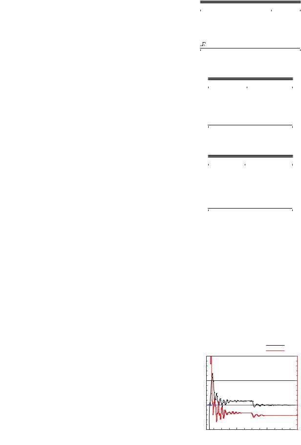
Fig. 1 Typical lift and drag convergence, M∞ 0.85, Re 5 × 10⁶, CL 0.5, k-kL turbulence model.
Downloaded by 94.180.100.60 on November 25, 2018 | http://arc.aiaa.org | DOI: 10.2514/1.C034481
1460 |
|
|
ABDOL-HAMID ET AL. |
|
|
|
|
|
|
No limiter |
|
|
No limiter |
||
0.0265 |
|
-0.07 |
|
h-minmod limiter |
|||
|
h-minmod limiter |
|
|||||
|
|
|
|
|
|
||
0.0260 |
|
|
|
-0.08 |
|
|
|
D |
|
|
|
m |
|
|
|
C |
|
|
|
C |
|
|
|
0.0255 |
|
|
|
-0.09 |
|
|
|
0.0250 |
0.000005 |
0.000010 |
0.000015 |
-0.10 |
0.000005 |
0.000010 |
0.000015 |
0.000000 |
0.000000 |
||||||
|
h2 |
|
|
|
|
h2 |
|
a) Coefficient of drag |
|
|
b) Coefficient of pitching moment |
|
|||
|
|
2.80 |
|
No limiter |
|
|
|
|
|
|
|
|
|
|
|
|
|
|
|
h-minmod limiter |
|
|
|
|
|
2.75 |
|
|
|
|
|
|
(deg) |
2.70 |
|
|
|
|
|
|
2.65 |
|
|
|
|
|
|
|
α |
|
|
|
|
|
|
|
|
|
|
|
|
|
|
|
|
2.60 |
|
|
|
|
|
|
|
2.55 |
|
|
|
|
|
|
|
2.50 |
0.000005 |
0.000010 |
0.000015 |
|
|
|
|
0.000000 |
|
|
|||
|
c) Angle of attack, deg |
h2 |
|
|
|
||
|
|
|
|
|
|||
Fig. 2 Effects of limiter as a function of characteristic grid spacing, CL 0.5, k-kL turbulence model. |
|||||||
0.030 |
|
No limiter |
0.60 |
|
No limiter |
||
|
h-minmod limiter |
|
h-minmod limiter |
||||
|
|
Venkat limiter |
|
|
Venkat limiter |
||
0.029 |
|
|
|
0.58 |
|
|
|
|
|
|
|
|
|
|
|
0.028 |
|
|
|
0.56 |
|
|
|
|
|
|
|
|
|
|
|
D |
|
|
|
L |
|
|
|
C |
|
|
|
C 0.54 |
|
|
|
0.027 |
|
|
|
0.52 |
|
|
|
|
|
|
|
|
|
|
|
0.026 |
|
|
|
0.50 |
|
|
|
|
|
|
|
|
|
|
|
0.025 |
0.000005 |
0.000010 |
0.000015 |
0.48 |
0.000005 |
0.000010 |
0.000015 |
0.000000 |
0.000000 |
||||||
|
h2 |
|
|
|
h2 |
|
|
a) Drag coefficient |
|
|
b) Lift coefficient |
|
|
||
|
|
|
|
No limiter |
|
|
|
|
|
|
|
h-minmod limiter |
|
|
|
|
|
|
|
Venkat limiter |
|
|
|
|
|
-0.08 |
|
|
|
|
|
|
m |
|
|
|
|
|
|
|
C |
|
|
|
|
|
|
|
|
-0.10 |
|
|
|
|
|
-0.12 |
0.000005 |
0.000010 |
0.000015 |
0.000000 |
h2
c) Pitching moment coefficient
Fig. 3 Effects of limiter as a function of characteristic grid spacing, α 2.75 deg, k-kL turbulence model.

Downloaded by 94.180.100.60 on November 25, 2018 | http://arc.aiaa.org | DOI: 10.2514/1.C034481
ABDOL-HAMID ET AL. |
1461 |
The solution at each time step is updated with a backward Euler time-integration scheme. At each time step, the linear system of equations is approximately solved with a multicolor point-implicit procedure [25]. Local time-step scaling is employed to accelerate convergence to steady state. For turbulent flows, a variety of turbulence models are available within FUN3D. The k-kL model [7] used in this study is a linear eddy-viscosity two-equation turbulence model, which is solved in a loosely coupled approach with the meanflow equations. The nonlinear quadratic constitutive relation (QCR) developed by Spalart [26] will also be used to compute the Reynolds stress terms. This will be referred to as QCR nonlinear option used by k-kL [7]. The discretization of the turbulence model diffusion terms is handled in the same fashion as the mean-flow viscous terms.
IV. Focus Cases from DPW-VI and Results
In the present paper, we will cover the effect of limiter and turbulence model formulations in the computational results of CRM WB configuration for a number of test cases at M∞ 0.85 and Re 5 × 10⁶:
1)CRM grid convergence study (CL 0.5): CRM WB configurations computed with k-kL including reconstruction limiter effects;
2)CRM grid convergence study (α 2.75 deg): CRM WB configurations computed with k-kL including reconstruction limiter effects; and
3)CRM WB static aeroelastic effect: angle-of-attack sweep computed with k-kL, both linear eddy-viscosity and QCR variations.
|
No limiter |
|
-1.5 |
h-minmod limiter |
|
|
Venkat limiter |
|
|
= 0.131, Experimental Data |
|
-1.0 |
|
|
-0.5 |
|
|
p |
|
|
C |
|
|
0.0 |
|
|
0.5 |
|
|
1.0 |
0.5 |
1 |
0 |
||
|
x / c |
|
|
No limiter |
|
-1.5 |
h-minmod limiter |
|
|
Venkat limiter |
|
|
0.131, Experimental Data |
|
-1.0 |
|
|
-0.5 |
|
|
p |
|
|
C |
|
|
0.0 |
|
|
0.5 |
|
|
1.0 |
0.5 |
1 |
0 |
||
|
x / c |
|
a) = 0.131, medium grid |
b) = 0.131, ultrafine grid |
|
No limiter |
|
-1.5 |
h-minmod limiter |
|
|
Venkat limiter |
|
|
= 0.502, Experimental Data |
|
-1.0 |
|
|
-0.5 |
|
|
p |
|
|
C |
|
|
0.0 |
|
|
0.5 |
|
|
1.0 |
0.5 |
1 |
0 |
||
|
x / c |
|
|
No limiter |
|
-1.5 |
h-minmod limiter |
|
|
Venkat limiter |
|
|
0.502, Experimental Data |
|
-1.0 |
|
|
-0.5 |
|
|
p |
|
|
C |
|
|
0.0 |
|
|
0.5 |
|
|
1.0 |
0.5 |
1 |
0 |
||
|
x / c |
|
c) = 0.502, medium grid |
d) = 0.502, ultrafine grid |
-1.5 |
No limiter |
|
h-minmod limiter |
|
|
|
Venkat limiter |
|
|
= 0.95, Experimental Data |
|
-1.0 |
|
|
-0.5 |
|
|
p |
|
|
C |
|
|
0.0 |
|
|
0.5 |
|
|
1.0 |
0.5 |
1 |
0 |
||
|
x / c |
|
|
No limiter |
|
-1.5 |
h-minmod limiter |
|
|
Venkat limiter |
|
|
0.95, Experimental Data |
|
-1.0 |
|
|
-0.5 |
|
|
p |
|
|
C |
|
|
0.0 |
|
|
0.5 |
|
|
1.00 |
0.5 |
1 |
|
x / c |
|
e) = 0.95, medium grid |
f) = 0.95, ultrafine grid |
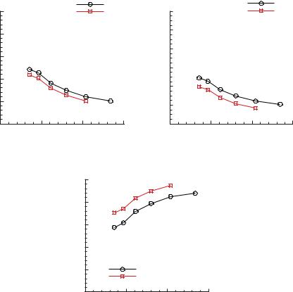
Fig. 4 Comparison of chordwise surface pressure coefficient distributions, α 2.75 deg, k-kL turbulence model.
Downloaded by 94.180.100.60 on November 25, 2018 | http://arc.aiaa.org | DOI: 10.2514/1.C034481
1462 |
ABDOL-HAMID ET AL. |
The first and third cases are based on the required cases from DPW-VI. The second case is a traditional grid convergence study where all flow conditions are fixed, including angle of attack.
The current FUN3D solutions were computed on mixed-element unstructured grids provided by the DPW committee. These grids were generated using the gridding guidelines specified for the workshop (see footnote ¶). Table 2 lists the grid sizes for the family of grids used for the grid convergence study. These grids have prismatic cells near the solid surface of the wing/body and tetrahedral cells away from the wall with a small number of pyramids in the interface region between the prisms and tetrahedral cells. Table 3 lists the grids used for the angle-of-attack sweeps. These grids are at the medium grid level and have a similar topology as those created for the grid convergence study. Recall that these grid geometries include the static aeroelastic twist and deformation experienced by the model at different angles of attack, but omit the model support features and tunnel walls. All the force and moment coefficients presented herein are the total value (combined pressure and viscous components) for the wing and body. Computed results will be compared with experimental data for CL, CD, Cm, and CP from run 197R44 (see footnote **) from the National Transonic Facility test at NASA Langley Research Center. We will also compare CFD with experimental data [27] that were generated with a pressure-sensitive paint measuring technique done at the NASA Ames 11 ft transonic tunnel. As mentioned earlier, the CFD model did not include support system or tunnel walls.
A. Constant Lift Grid Convergence Study
started at α 2.75 deg to get initially converged solutions. Then, the angle of attack is automatically adjusted to reach the target lift coefficient within 0.0001. Figure 1 shows a typical total lift and drag coefficient convergence history through the two-step solution process. FUN3D takes approximately 6000 iterations to complete the entire process, targeting CL 0.5.
Drag coefficient CD and pitching moment coefficient Cm are plotted as a function of a characteristic grid spacing squared h2 in Figs. 2a and 2b, respectively. The h2 is computed as the number of nodes N raised to the −2∕3 power. This exponent is based on two assumptions: 1) the characteristic length of the grid spacing varies with the cube root of the cell volume, and 2) the solution lies within the “asymptotic range” of grid convergence and its spatial error decreases with second-order accuracy. When these assumptions are met, the computed outputs should vary linearly with h2. On the finer grids, the difference between no limiter and h-minmod generally diminishes for the values shown in Fig. 2. The CD values of the finest grid with no limiter and h-minmod are within one count, 0.0001. The Cm values of the finest grid with no limiter and h-minmod are within 0.001. The angle of attack required for CL 0.5 is also plotted as a function of h2 in Fig. 2c. This trim angle of attack decreases for both methods as the grid is refined. This decrease in angle of attack with grid refinement at constant coefficient of lift is analogous to an increase in coefficient of lift with grid refinement at constant α. The h-minmod limiter reduces the differences between tiny and ultrafine grids by more than 50% (compared with no limiter) for all the values plotted in Fig. 2.
One of the required cases computed for |
DPW-VI is a grid |
|
|
B. Constant Angle-of-Attack Grid Convergence Study |
|||||||||||
convergence |
study performed at the design condition of M |
∞ |
|
0.85 |
, |
|
|
|
An alternate grid convergence study fixes geometry and all flow |
||||||
6 |
|
|
|
|
|
|
|
||||||||
Re 5 × 10 |
|
, and CL 0.5 for the WB configuration. Each case is |
|
|
conditions (independent variables) to evaluate the effect of grid in |
||||||||||
|
|
|
|
|
|
k-kL |
|
|
|
|
|
|
|
k-kL |
|
|
|
0.030 |
|
|
|
k-kL+QCR |
|
|
|
0.60 |
|
|
k-kL+QCR |
||
|
|
0.029 |
|
|
|
|
|
|
|
|
|
0.58 |
|
|
|
|
|
|
|
|
|
|
|
|
|
|
|
|
|
|
|
|
|
0.028 |
|
|
|
|
|
|
|
|
|
0.56 |
|
|
|
|
|
|
|
|
|
|
|
|
|
|
|
|
|
|
|
|
|
D |
|
|
|
|
|
|
|
L |
0.54 |
|
|
|
|
|
|
C |
|
|
|
|
|
|
|
C |
|
|
|
|
|
|
|
0.027 |
|
|
|
|
|
|
|
|
|
0.52 |
|
|
|
|
|
|
|
|
|
|
|
|
|
|
|
|
|
|
|
|
|
0.026 |
|
|
|
|
|
|
|
|
|
0.50 |
|
|
|
|
|
|
|
|
|
|
|
|
|
|
|
|
|
|
|
|
|
0.025 |
0.000005 |
0.000010 |
0.000015 |
|
|
|
0.48 |
0.000005 |
0.000010 |
0.000015 |
|||
|
|
0.000000 |
|
|
|
0.000000 |
|||||||||
|
|
|
h2 |
|
|
|
|
|
|
|
|
|
h2 |
|
|
|
|
a) Drag coefficient |
|
|
|
|
|
|
b) Lift coefficient |
|
|
||||
|
|
|
|
-0.07 |
|
|
|
|
|
|
|
|
|
|
|
|
|
|
|
-0.08 |
|
|
|
|
|
|
|
|
|
|
|
|
|
|
|
-0.09 |
|
|
|
|
|
|
|
|
|
|
|
|
|
|
|
m |
|
|
|
|
|
|
|
|
|
|
|
|
|
|
C |
|
|
|
|
|
|
|
|
|
|
|
|
|
|
|
|
-0.10 |
|
|
|
|
|
|
|
|
|
|
|
|
|
|
|
-0.11 |
|
|
|
|
k-kL |
|
|
|
|
||
|
|
|
|
|
|
|
|
|
k-kL+QCR |
|
|
|
|||
|
|
|
|
-0.12 |
|
|
0.000005 |
|
0.000010 |
0.000015 |
|
|
|||
|
|
|
|
0.000000 |
|
|
|
|
|||||||
h2 c) Pitching moment coefficient
Fig. 5 Effect of QCR as a function of characteristic grid spacing, α 2.75 deg, no limiter, k-kL turbulence model.

Downloaded by 94.180.100.60 on November 25, 2018 | http://arc.aiaa.org | DOI: 10.2514/1.C034481
ABDOL-HAMID ET AL. |
1463 |
predicting flow quantities, such as surface pressure coefficient and total force coefficients (dependent variables). The grids provided by the DPW-VI committee are based on the geometry at α 2.75 deg, which is close to the design condition for the CRM WB configuration.
The first set of results evaluates the effect of limiters when using the basic linear k-kL turbulence model. Drag, lift, and moment coefficients as well as surface pressure coefficients at different locations on the wing are assessed. The basic no-limiter results are compared with the Venkat and the h-minmod limiter results. The lift, drag, and moment coefficients are plotted as a function of h2 in Figs. 3a–3c, respectively. On the finer grids, the differences between no limiter, Venkat limiter, and h-minmod limiter diminish.
The CD values on the finest grid are within about five counts, 0.0005, for the various methods. The CL values of the finest grid are within about 0.008, and the Cm values of the finest grid are within about 0.005. As the grid is refined, CD and CL increase for either no limiter or h-minmod and decrease for the Venkat limiter. The opposite occurs for Cm. In other words, the Venkat limiter has a different trend than the other approaches. This different trend between the limiters with grid refinement causes 10% differences between the results at the medium grid level (h2 ≈ 0.000008). The medium grid level is usually built to compute the required cases close to design condition (α 2.50–4.00 deg) with an “industry standard” acceptable level of accuracy. However, the large influence of the limiter on the medium grid level (over 44 million nodes) indicates
|
k-kL |
|
k-kL |
-1.5 |
k-kL+QCR |
-1.5 |
k-kL+QCR |
|
0.131, Experimental Data |
|
0.131, Experimental Data |
|
-1.0 |
|
|
|
-1.0 |
|
|
|
-0.5 |
|
|
|
-0.5 |
|
|
p |
|
|
|
p |
|
|
|
C |
|
|
C |
|
|
||
|
0.0 |
|
|
|
0.0 |
|
|
|
0.5 |
|
|
|
0.5 |
|
|
|
1.0 |
0.5 |
1 |
|
1.0 |
0.5 |
1 |
|
0 |
|
0 |
||||
|
|
x / c |
|
|
|
x / c |
|
a) |
= 0.131, medium grid |
|
b) |
= 0.131, ultrafine grid |
|
||
|
|
k-kL |
|
|
|
k-kL |
|
|
-1.5 |
k-kL+QCR |
|
|
-1.5 |
k-kL+QCR |
|
|
|
0.502, Experimental Data |
|
|
0.502, Experimental Data |
||
|
-1.0 |
|
|
|
-1.0 |
|
|
|
-0.5 |
|
|
|
-0.5 |
|
|
p |
|
|
|
p |
|
|
|
C |
|
|
C |
|
|
||
|
0.0 |
|
|
|
0.0 |
|
|
|
0.5 |
|
|
|
0.5 |
|
|
|
1.0 |
0.5 |
1 |
|
1.0 |
0.5 |
1 |
|
0 |
|
0 |
||||
|
|
x / c |
|
|
|
x / c |
|
c) |
= 0.502, medium grid |
|
d) |
= 0.502, ultrafine grid |
|
||
|
|
k-kL |
|
|
|
k-kL |
|
|
-1.5 |
k-kL+QCR |
|
|
-1.5 |
k-kL+QCR |
|
|
|
0.95, Experimental Data |
|
|
0.95, Experimental Data |
||
|
-1.0 |
|
|
|
-1.0 |
|
|
|
-0.5 |
|
|
|
-0.5 |
|
|
p |
|
|
|
p |
|
|
|
C |
|
|
C |
|
|
||
|
0.0 |
|
|
|
0.0 |
|
|
|
0.5 |
|
|
|
0.5 |
|
|
|
1.0 |
0.5 |
1 |
|
1.0 |
0.5 |
1 |
|
0 |
|
0 |
||||
|
|
x / c |
|
|
|
x / c |
|
e) = 0.95, medium grid |
f) = 0.95, ultrafine grid |
Fig. 6 Comparison of surface pressure coefficient distributions, turbulence model variation, α 2.75 deg, no limiter.
Downloaded by 94.180.100.60 on November 25, 2018 | http://arc.aiaa.org | DOI: 10.2514/1.C034481
1464 |
ABDOL-HAMID ET AL. |
|
the likelihood that this grid is still not yet fine enough for many |
grid solutions. At the medium grid level, the no limiter and h-minmod |
|
engineering purposes. |
|
limiter give similar results at all stations, which are different than the |
Next, chordwise surface pressure coefficients from the medium |
Venkat limiter results as shown in Fig. 4a, 4c, and 4e. Overall, both |
|
and ultrafine grid solutions are examined. Figure 4 shows surface |
no-limiter and h-minmod limiter results are much closer to the |
|
pressure coefficients at three span locations: η 0.131, 0.502, |
experimental pressure data (see footnote **) as compared with the |
|
and 0.95. Figures 4a, 4c, and 4e show results from the medium grid |
Venkat limiter results. However, this does not necessarily mean that |
|
solutions, whereas Figs. 4b, 4d, and 4f show results from the ultrafine |
they are more accurate, because numerical errors due to insufficient |
|
Cfx
a) α = 2.75 deg |
b) α = 3.00 deg |
c) α = 3.25 deg |
d) α = 3.50 deg |
e) α = 3.75 deg |
f) α = 4.00 deg |
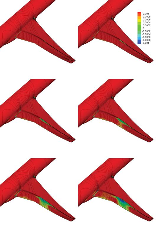
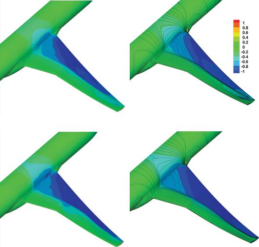
Fig. 7 Streamwise component of skin friction color contours and coefficient of pressure contour lines, k-kL turbulence model, no limiter.
Downloaded by 94.180.100.60 on November 25, 2018 | http://arc.aiaa.org | DOI: 10.2514/1.C034481
ABDOL-HAMID ET AL. |
1465 |
grid refinement may still be playing a large role. In fact, all three approaches are much closer to each other at the ultrafine grid level, as shown in Figs. 4b, 4d, and 4f. The difference is slightly wider at η 0.95 toward the wing tip, but diminished from the medium grid levels. The surface pressure results are consistent with what was discussed for CD and CL in Fig. 3. At the ultrafine grid level, CD and CL are within less than 1% between all the approaches.
The basic (linear) k-kL results are compared with (nonlinear) k-kL QCR turbulence model results in Fig. 5. These solutions were computed without a limiter. The drag coefficient CD, lift coefficient CL, and moment coefficient Cm are plotted as a function of h2 in Figs. 5a–5c, respectively. The variation in CL, CD, and Cm with grid refinement shows similar trends for both k-kL and k-kL QCR. The differences are very consistent across the grid levels, with k-kL QCR resulting in a smaller CL and CD and higher (less negative) Cm than the basic k-kL model.
The corresponding surface pressure coefficients from the medium and ultrafine grid solutions are shown in Fig. 6 at η 0.131, 0.502, and 0.95. Figures 6a, 6c, and 6e are the results from the medium grid solutions. Figures 6b, 6d, and 6f are the results on the ultrafine grid level. Overall, results from the linear and nonlinear turbulence models are very similar for η 0.131 and 0.502, with a slight difference at the η 0.95 station.
C. Angle-of-Attack Sweep Study : α 2.50–4.00 deg
One of the required cases computed for DPW-VI is an angle-of- attack sweep study, performed at the design condition of M∞ 0.85
and Re 5 × 10⁶ for the WB configuration. Results and analysis in the current section focus on a range of angles of attack for this case near the design lift coefficient (α 2.50–4.00 deg). The majority of the results presented for this angle-of-attack sweep use the medium grid node-centered grids provided by the DPW-VI committee for this case, as listed in Table 3. A subset of solutions (α 2.75, 3.25, and 4.00 deg) are computed on the ultrafine grid provided for the grid convergence study, as listed in Table 2.
As with the grid convergence studies, the effects of different limiters and QCR are assessed. Qualitatively, the solutions between these different numerical approaches are very similar. Typical results of skin friction coefficient color contours and pressure coefficient contour lines (0.1 increments) are shown in Fig. 7. The results shown in Fig. 7 are for the basic k-kL turbulence model and no-limiter approach on the medium grids. A primary wing shock is indicated on the upper surface of the wing by the clustering of pressure coefficient contour lines that parallel the wing trailing edge. The series of subplots in Fig. 7 detail the attached flow regions and growing separation regions colored by blue shade (negative skin friction). There is no indication of separated flow for α < 3.75 deg. A small area of separated flow is observed in the midspan of the wing just aft of the primary shock for α < 3.75 deg. The skin friction coefficient is also low in the wing–root junction region behind the intersection of the primary wing shock and the fuselage.
Figure 8 shows a qualitative comparison of computed surface pressure coefficient contours and experimental data [27] at α 3.00 and 4.00 deg. These typical computational results are also for the
Cp
a) α = 3.00 deg, Experiment |
b) α = 3.00 deg, CFD |
c) α = 4.00 deg, Experiment |
d) α = 4.00 deg, CFD |
Fig. 8 Comparison of pressure coefficient contours between computation (k-kL with no limiter) and experiment [27].
Downloaded by 94.180.100.60 on November 25, 2018 | http://arc.aiaa.org | DOI: 10.2514/1.C034481
1466
|
0.75 |
|
0.70 |
|
0.65 |
L |
0.60 |
C |
|
|
0.55 |
|
0.50 |
|
0.45 |
ABDOL-HAMID ET AL.
No limiter, medium grid h-minmod limiter, medium grid Venkat limiter, medium grid No limiter, ultra grid Experimental Data 
2.5 |
3.0 |
3.5 |
4.0 |
α (deg)
CL
|
No limiter, medium grid |
|
0.75 |
h-minmod limiter, medium grid |
|
Venkat limiter, medium grid |
||
|
||
|
No limiter, ultra grid |
|
0.70 |
Experimental Data |
|
|
0.65 

0.60
0.55
0.50
0.45 


 -0.12 -0.10 -0.08 -0.06 -0.04 -0.02
Cm
a) Lift coefficient with respect to angle of attack |
b) Lift coefficient with respect to pitching |
|
moment coefficient |
|
0.75 |
|
|
|
|
|
|
|
0.70 |
|
|
|
|
|
|
L |
0.65 |
|
|
|
|
||
0.60 |
|
|
|
C |
|
|
|
|
|
||
|
0.55 |
|
|
|
|
|
|
|
0.50 |
|
|
|
|
|
|
|
0.45 |
|
|
|
|
|
|
|
0.02 |
||
No limiter, medium grid h-minmod limiter, medium grid Venkat limiter, medium grid No limiter, ultra grid Experimental Data 
0.03 |
0.04 |
0.05 |
CD
CL
|
No limiter, medium grid |
|
0.75 |
h-minmod limiter, medium grid |
|
Venkat limiter, medium grid |
||
|
||
|
No limiter, ultra grid |
|
0.70 |
Experimental Data |
|
|
0.65
0.60
0.55
0.50
0.45 |
0.02 |
0.03 |
0.04 |
0.05 |
0.01 |
CDi
c) Lift coefficient with respect to drag coefficient |
d) Lift coefficient with respect to idealized drag |
|
coefficient |
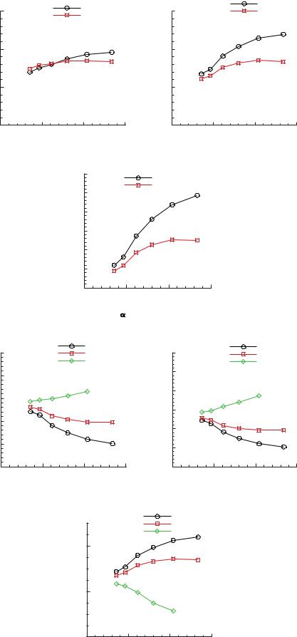
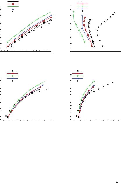
Fig. 9 Effect of limiters, k-kL turbulence model.
basic k-kL turbulence model and no-limiter approach on the medium grids. The experimental data [27] are generated with a pressuresensitive paint measurement technique at the NASA Ames 11 ft transonic tunnel. The experimental results in Fig. 8 show no clear indication of significant separated flow on the upper surface of the wing behind the primary shock or in the wing–root juncture region at these angles of attack. The computed results are qualitatively comparable and consistent with experimental data behavior. The computed shock on the outboard wing does appear to be slightly stronger and farther aft than what is indicated by the experimental data. This is consistent with the trend shown in the preceding section for the constant angle-of-attack grid convergence study. Although not shown here, other approaches used in the present paper gave similar CFD behavior and consistency with experimental data at these angles of attack.
1. Effect of Limiters
Figure 9 shows a comparison of computed lift and drag polars in α 0.25 deg increments. Computed results with different limiters (no limiter, h-minmod, and Venkat) options on the medium grids are shown, and the experimental data (see footnote **) are included for reference. As noted in the preceding section, all computed results show very similar trends and no indication of separated flow. This is in contrast to the FUN3D trends with the SA turbulence model in DPW-V for full viscous terms [6]. The SA results from [6] showed an abrupt reduction in CL and CD for α > 3.00 deg, which was delayed and reduced by the use of a limiter or eliminated with a thin-layer viscous term approximation. This early stall was correlated to a massive separation bubble generated at the root of the wing initiated at a forward shock location [6].
In Figs. 9a–9c, the medium grid computed results with the Venkat limiter produce the highest CL and the lowest CD and Cm
(at constant lift), and no-limiter results produce the lowest CL and the highest CD and Cm. This is the same trend for CL and Cm shown in the preceding section for the constant angle-of-attack grid convergence study (see Fig. 3), but the trend for CD is different depending on whether the computations are at a fixed lift or fixed angle of attack. In any case, these results reinforce the claim that the medium grids are not fine enough. Figure 9d shows the idealized drag coefficient as a function of CL, where 


 . Similar trends are exhibited as in Fig. 9c. The ultrafine grid results shown in Fig. 9 give an indication of the effect of grid refinement, although it is important to note that the aeroelastic effects included in this grid are only consistent for the α 2.75 deg case.
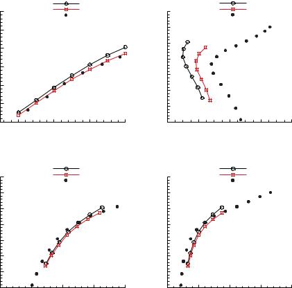
2. Effect of Turbulence Model
Figure 10 shows a comparison of computed lift and drag polars in α 0.25 deg increments. Computed results with different variations of k-kL (k-kL and k-kL QCR) on the medium grids are shown, and the experimental data (see footnote **) are again included for reference. As noted in a prior section, all computed results show very similar trends and no indication of separated flow. The linear k-kL results shows slightly higher CL and lower Cm and CD (at constant lift) than k-kL QCR results, with the differences increasing with CL. The k-kL QCR results are closer to experimental data than the basic k-kL turbulence model for CL and Cm; based on the results in Fig. 5, this is expected to be true also for finer grids (both sets of results will move away from experiment as the grid is refined). Neither model can be considered to be closer to experiment for CD and CDi, although the k − kL QCR polar shapes are somewhat better than those predicted by k-kL. Note that the k-kL QCR model allowed the use of higher Courant–Friedrichs–Lewy numbers for the solutions of both the meanflow and turbulence model equations.
Downloaded by 94.180.100.60 on November 25, 2018 | http://arc.aiaa.org | DOI: 10.2514/1.C034481
ABDOL-HAMID ET AL. |
1467 |
|
|
|
k-kL |
|
|
|
|
k-kL |
|
|
0.75 |
|
k-kL+QCR |
|
0.75 |
|
|
k-kL+QCR |
|
|
|
|
Experimental Data |
|
|
|
Experimental Data |
||
|
0.70 |
|
|
|
0.70 |
|
|
|
|
|
|
|
|
|
|
|
|
|
|
|
0.65 |
|
|
|
0.65 |
|
|
|
|
|
|
|
|
|
|
|
|
|
|
L |
|
|
|
|
0.60 |
|
|
|
|
0.60 |
|
|
|
L |
|
|
|
|
|
C |
|
|
|
C |
|
|
|
|
|
|
|
|
|
|
0.55 |
|
|
|
|
|
0.55 |
|
|
|
0.50 |
|
|
|
|
|
|
|
|
|
|
|
|
|
|
|
0.50 |
|
|
|
0.45 |
|
|
|
|
|
|
|
|
|
|
|
|
|
|
|
0.45 |
3 |
3.5 |
4 |
0.40 |
-0.08 |
-0.06 |
-0.04 |
-0.02 |
|
2.5 |
-0.1 |
|||||||
|
|
α (deg) |
|
|
|
|
Cm |
|
|
a) Lift coefficient with respect to angle of attack |
b) Lift coefficient with respect to pitching moment |
||||||||
|
|
|
|
|
coefficient |
|
|
|
|
|
|
|
k-kL |
|
|
|
|
k-kL |
|
0.75 |
|
|
k-kL+QCR |
|
0.75 |
|
|
k-kL+QCR |
|
|
|
|
Experimental Data |
|
|
|
Experimental Data |
||
0.70 |
|
|
|
|
0.70 |
|
|
|
|
0.65 |
|
|
|
|
0.65 |
|
|
|
|
0.60 |
|
|
|
|
0.60 |
|
|
|
|
L |
|
|
|
|
L |
|
|
|
|
C |
|
|
|
|
C |
|
|
|
|
0.55 |
|
|
|
|
0.55 |
|
|
|
|
0.50 |
|
|
|
|
0.50 |
|
|
|
|
0.45 |
|
|
|
|
0.45 |
|
|
|
|
0.40 |
0.02 |
0.03 |
0.04 |
0.05 |
0.40 |
0.02 |
0.03 |
0.04 |
0.05 |
0.01 |
0.01 |
||||||||
|
|
CD |
|
|
|
|
CDi |
|
|
c) Lift coefficient with respect to drag coefficient |
d) Lift coefficient with respect to idealized drag |
||||||||
coefficient
Fig. 10 Effect of turbulence model, medium grid, α ≤ 4.00, no limiter, k-kL turbulence model.
V.Conclusions
The FUN3D computational fluid dynamics code was applied to the DPW-VI Common Research Model configuration, with the k-kL-MEAH2015 turbulence model as well as with a nonlinear quadratic constitutive relation (QCR) variant of the same model. The effect of reconstruction limiter was explored by running cases with no limiter, with a stencil-based min-mod limiter augmented with a heuristic pressure limiter, and with the Venkat limiter. Two different grid refinement studies (one at constant lift and one at constant angle of attack) showed significant (up to 10%) differences between results on the medium grid, depending on the choice of limiter (or no limiter). Lift coefficient predictions with no limiter or the h-minmod limiter both increased with grid refinement, whereas they decreased with the Venkat limiter. However, results generally approached each other with grid refinement, as expected. The large differences between results on the medium grid indicate that this grid level is too coarse for drawing conclusions in comparison with experiment.
The linear k-kL-MEAH2015 model generally showed trends consistent with the experiment, with no evidence of the large corner separation (and early stall) that plagues many other linear models, even as high as α 4 deg. Including the QCR in the model had only a relatively minor effect; its results were also reasonably good compared with experiment.
Acknowledgment
This research was sponsored by NASA’s Transformational Tools and Technologies Project of the Transformative Aeronautics Concepts Program under the Aeronautics Research Mission Directorate.
References
[1]Biedron, R. T., et al., “FUN3D Manual: 12.9,” NASA Langley Research Center, NASA TM-2015-219012, Hampton, VA, Feb. 2016.
[2]Anderson, W., and Bonhaus, D., “An Implicit Upwind Algorithm for Computing Turbulent Flows on Unstructured Grids,” Computers and Fluids, Vol. 23, No. 1, 1994, pp. 1–21. doi:10.1016/0045-7930(94)90023-X
[3]Anderson, W. K., Rausch, R. D., and Bonhaus, D. L., “Implicit/ Multigrid Algorithm for Incompressible Turbulent Flows on Unstructured Grids,” Journal of Computational Physics, Vol. 128, No. 2, 1996, pp. 391–408.
doi:10.1006/jcph.1996.0219
[4]Nielsen, E. J., “Aerodynamic Design Sensitivities on an Unstructured Mesh Using the Navier–Stokes Equations and a Discrete Adjoint Formulation,” Ph.D. Thesis, Virginia Polytechnic Inst. and State Univ., Blacksburg, VA, 1998.
[5]Lee-Rausch, E. M., Hammond, D. P., Nielsen, E. J., Pirzadeh, S. Z., and Rumsey, C. L., “Application of the FUN3D Solver to the 4th AIAA Drag Prediction Workshop,” Journal of Aircraft, Vol. 51, No. 4, 2014,
pp.1149–1160. doi:10.2514/1.C032558
[6]Park, M. A., Laflin, K. R., Chaffin, M. S., Powell, N., and Levy, D. W., “CFL3D, FUN3D, and NSU3D Contributions to the Fifth Drag Prediction Workshop,” Journal of Aircraft, Vol. 51, No. 4, 2014, pp. 1268–1283. doi:10.2514/1.C032613
[7]Abdol-Hamid, K. S., Carlson, J.-R., and Rumsey, C. L., “Verification and Validation of the k-kL Turbulence Model in FUN3D and CFL3D Codes,” AIAA Paper 2016-3941, June 2016.
[8]Menter, F. R., “Two-Equation Eddy-Viscosity Turbulence Models for Engineering Applications,” AIAA Journal, Vol. 32, No. 8, 1994,
pp.1598–1605.
doi:10.2514/3.12149
[9]Vassberg, J. C., DeHaan, M. A., Rivers, S. M., and Wahls, R. A., “Development of a Common Research Model for Applied CFD Validation Studies,” AIAA Paper 2008-6919, June 2008.