

1_c034239
.pdfDownloaded by 94.180.100.60 on November 25, 2018 | http://arc.aiaa.org | DOI: 10.2514/1.C034239
JOURNAL OF AIRCRAFT
Vol. 54, No. 5, September–October 2017
Controlling Limit Cycle Oscillation Amplitudes in Nonlinear
Aeroelastic Systems
Himanshu Shukla and Mayuresh J. Patil†
Virginia Polytechnic Institute and State University, Blacksburg, Virginia 24060
DOI: 10.2514/1.C034239
The paper focuses on the design of nonlinear state feedback controllers to minimize the amplitude of limit cycle oscillations exhibited by nonlinear aeroelastic systems. Nonlinear normal modes are computed for the closed-loop system to represent the flutter mode dynamics using a single mode. The effectiveness of nonlinear normal modes as a tool to capture the limit cycle oscillation growth is demonstrated. The harmonic balance method is used to estimate the amplitude and frequency of the limit cycle oscillations exhibited by the flutter mode. Analytical estimates of sensitivities of limit cycle amplitude with respect to the introduced control parameters are derived and shown to match closely to the sensitivities computed numerically using the finite difference method on a time marching simulation of the complete aeroelastic system. A multi-objective optimization problem that minimizes the estimate of limit cycle oscillation amplitude and an approximate measure of control cost is solved using the analytical sensitivities. Numerical simulation results are used to verify that minimizing the estimate of the limit cycle amplitude of the flutter nonlinear normal mode corresponds closely to minimizing the simulated limit cycle amplitude of the complete aeroelastic system.
|
|
|
Nomenclature |
|
a |
|
= location of elastic axis |
||
Gα |
|
= coefficient of nonlinear stiffness term |
||
|
|
= nondimensional plunge displacement, m |
||
h |
|
|||
Iα |
|
= moment of inertial along the pitch degree of freedom, |
||
|
|
|
kg m2 |
|
= nondimensional aerodynamic force and moment |
||||
L, |
M |
|||
m |
|
= |
mass, kg |
|
rα |
|
= dimensionless radius of gyration |
||
T4, T10 |
= two of Theodorsen’s coefficients |
|||
t |
|
= |
time, s |
|
u |
|
= |
nondimensional freestream velocity |
|
xα |
|
= |
dimensionless static imbalance |
|
α= pitch angle, rad
β= control input, trailing-edge flap deflection
μ= density ratio
ω |
= |
ratio of plunge to pitch natural frequency |
ωh, ωα |
= |
natural frequency along plunge and pitch degree of |
|
|
freedom |
I.Introduction
AEROELASTIC systems are inherently nonlinear, thereby exhibiting quite diverse response phenomena. A combination of geometric, freeplay, structural, and aerodynamic nonlinearities
lead to complex behaviors [1–3], including the existence of multiple equilibria, bifurcations, chaos [4], limit cycle oscillations (LCOs), and various types of resonances [5]. To enhance the flight envelope and increase the maneuverability of aerial vehicles, suppression of such undesired phenomena is quite critical and has been a topic of active interest among researchers for the past few decades. Woolston et al. [6,7] and Shen [8] looked into the effects of structural nonlinearities on the flutter of a wing. An excellent review of the
Presented as Paper 2016-2004 at the AIAA Atmospheric Flight Mechanics Conference, San Diego, CA, 4–8 January 2016; received 2 October 2016; revision received 2 February 2017; accepted for publication 1 March 2017; published online Open Access 16 May 2017. Copyright © 2017 by Himanshu Shukla and Mayuresh Patil. Published by the American Institute of Aeronautics and Astronautics, Inc., with permission. All requests for copying and permission to reprint should be submitted to CCC at www.copyright.com; employ the ISSN 0021-8669 (print) or 1533-3868 (online) to initiate your request. See also AIAA Rights and Permissions www.aiaa.org/randp.
*Ph.D. Candidate, Aerospace and Ocean Engineering; hshukla@vt.edu.
†Associate Professor, Aerospace and Ocean Engineering; mpatil@vt.edu. Associate Fellow AIAA.
types of nonlinearities encountered in aeroelastic systems and their effects is given by Breitbach [9,10]. LCOs are constant amplitude and constant frequency periodic oscillations, the existence of which has been verified in experimental studies involving airfoil section models [11,12], as well as in modern aircraft such as the F-16 and F-18 [13]. The susceptibility of F/A-18 under certain store configurations to LCO was identified during the initial development and testing of the aircraft. An active oscillation control [14] system was augmented to the existing control system by the manufacturers, which used lateral acceleration feedback to drive the ailerons using a fixed, nonadaptive control law. Being subjected to LCOs over extended periods of time can cause structural fatigue, which might lead to system failure and catastrophic damage. This makes LCOs undesirable and their occurrence must be suppressed within the flight envelope.
Increasing the stiffness of the wing can postpone such instabilities to a certain extent with a disadvantage of decrease in performance. In contrast, active control strategies have been widely used in literature to improve performance with successful implementations to suppress flutter and LCOs. Noor and Venneri [15] gave a review of active control algorithms and wind-tunnel and flight-test results associated with feedback control and aeroelasticity. Lyons et al. [16] conducted a theoretical study of flutter suppression under full-state feedback using the Kalman estimator. Mukhopadhyay et al. [17] employed a nonlinear programming algorithm to search for an optimal control law based on the quadratic performance index. Gangsaas et al. [18] used a modified linear quadratic Gaussian methodology to develop control laws for gust load alleviation and flutter suppression. The unmeasurable states were defined using estimators in both cases. Karpel [19] formulated a partial-state feedback control law using pole placement techniques, whereas Horikawa and Dowell [20] used proportional gain feedback methods for gust load alleviation and flutter suppression. Even though the aforementioned works demonstrate the successful application of linear control theory to solve the aeroelastic instability problem, a need to develop more sophisticated aeroservoelastic models and controllers was recognized.
A review on active control of aeroelastic systems with nonlinearity is given by Mukhopadhyay [21–23]. A number of control approaches, ranging from traditional root locus and Nyquist plotbased methods [24] to nonlinear control [25–30], adaptive nonlinear control [31–39], L-1 adaptive control [40], robust control methods [41–47], and receptance-based control methods [48,49], have been used for flutter and LCO suppression in a typical wing section model with a single trailing-edge control surface and tested experimentally. An extended wing section model equipped with both a leadingand trailing-edge flap has also been used for the aeroelastic control problem [50–57].
1921

Downloaded by 94.180.100.60 on November 25, 2018 | http://arc.aiaa.org | DOI: 10.2514/1.C034239
1922 |
SHUKLA AND PATIL |
Some other methods focused on controlling bifurcations and achieving desirable effects in nonlinear systems have also been used. Abed and Fu [58,59] conducted a study of bifurcations of differential equations in the presence of control terms. Assuming that the uncontrolled system undergoes a bifurcation for a critical value of a certain system parameter, an investigation on the stabilizability of the system using quadratic and cubic terms was carried out. Abed and Wang [60] give a more general description for the control of bifurcation and chaos. Chen et al. [61,62] discuss a number of feedback design methods for the control of bifurcation and chaos along with various applications. Kang [63] designed a feedback law for delaying and stabilizing bifurcations using the method of normal forms [64], involving a state transformation and central manifold reduction. Similar methods have been used to control the LCO amplitudes for various nonlinear systems, for example, power systems [65], Van der Pol oscillator [66–68], and aeroelastic systems [69,70]. In general, the process involves predicting the LCO amplitude and using nonlinear state feedback control laws to modify the amplitude as desired. The method of normal forms [2,70–72], harmonic balance methods [73–76], and nonlinear normal modes [77–80] have been employed to predict the LCO amplitudes of nonlinear dynamic systems. Chen and Liu [81] used the homotopy analysis method to obtain algebraic equations that can be solved to obtain accurate estimates of LCO amplitudes and frequencies. Ghommem et al. [70] explore the use of linear and nonlinear static feedback control for control of LCO amplitudes. It is shown that linear control can delay the onset of flutter, whereas nonlinear control can be employed to efficiently control the LCO amplitudes.
The harmonic balance method derived by Krylov and Bogoliuboff [82] can be used to estimate LCO amplitudes and bifurcation behavior of nonlinear systems. Lee et al. [83] used harmonic balance to investigate the dynamic response of a two-degree-of-freedom airfoil section model coupled with a cubic nonlinearity. They obtained amplitude frequency relations and analyzed the stability of equilibrium points. A good correlation between the results from harmonic balance and numerical simulations was demonstrated. Yang and Zhao [84] analyzed the self-excited oscillations for a twodimensional wing model with nonlinear pitch stiffness using experimental data and the harmonic balance method. It is shown that the harmonic balance method is able to predict the unstable LCOs as well as the stable LCOs observed in the experimental data. Dimitriadis [73] used a combination of the harmonic balance method and numerical continuation techniques to study the bifurcation behavior of a two-dimensional airfoil section model in the presence of freeplay nonlinearity. Chen et al. [75] proposed an incremental harmonic balance method to analyze the aeroelastic problem in the presence of an external store.
Nonlinear normal modes (NNMs) [85–87] are an extension of the theory of linear normal modes for nonlinear systems. Emory and Patil [79] demonstrated that nonlinear normal modes can be used as an effective tool to predict the LCO amplitudes exhibited by an aeroelastic system. It is shown that the predictions of LCO amplitude obtained using NNMs are close to those obtained from time integration of the complete nonlinear aeroelastic system.
In the present work, the nonlinear flutter mode of the aeroelastic system is identified using the asymptotic method for computing NNMs. It is demonstrated that the existence of LCOs in aeroelastic systems can be explained using only the flutter NNM. This becomes very useful when considering higher order aeroelastic systems because their instability can be captured by a single NNM. The harmonic balance method is used to estimate the LCO amplitude of the flutter NNM and its sensitivities to the introduced control parameters. These are compared with actual sensitivities obtained numerically using the finite difference method and are shown to be accurate. Generating accurate analytical sensitivity equations using the harmonic balance method results in a reduction of computational effort in comparison to numerically estimating sensitivities from the finite difference method for large-scale systems. Also, the generated sensitivities are not prone to machine precision errors, which is always an issue when computing sensitivities using the finite difference method. A multi-objective optimization problem is solved
to minimize the estimated LCO amplitude of the flutter NNM and an approximate measure of control cost. It is shown that the optimal controller leads to a significant decrease in the estimated LCO amplitude of the flutter NNM, which corresponds to a similar reduction in the actual LCO amplitude obtained from the simulation of the complete aeroelastic system.
II.Nonlinear Aeroelastic System
Avariant of the typical airfoil section equipped with a trailing-edge flap is considered in the present work as shown in Fig. 1. The airfoil section is free to move up and down along the plunge degree of freedom and rotate in the pitch degree of freedom. The governing equations of motion can be obtained using Lagrange’s equations.
The nondimensional form of governing equations of motion [79] are expressed as
|
|
2 |
|
|
|
2 |
2 |
2 |
|
|
|
xαα |
ω |
|
rαα |
rα 1 |
Gαα |
(1) |
|||
h |
h −L |
xαh |
α M |
|||||||
These differ from the classic airfoil section equations given by Bisplinghoff et al. [88] in terms of the nonlinear stiffness term Gα.
The nondimensional plunge displacement, which is plunge |
|||
displacement |
h divided by the half chord b, is |
|
α is the pitch |
h; |
|||
angle; Iα is the pitch inertia; m is the mass; xα is the dimensionless static imbalance; ω ωh∕ωα is the plunge to pitch natural
frequency ratio, where ωh |
|
Kh∕m and ωα |
Kα∕Iα; rα is the |
||||||
|
|
|
p |
Iα∕mb |
2 |
|
p |
||
dimensionless |
radius of |
gyration |
|
|
; |
and the overdot |
|||
represents |
a |
derivative |
with |
respect |
to nondimensional time |
||||
|
p |
|
|
||||||
(τ tωα). |
|
|
|
|
|
|
|
|
|
L and M represent nondimensional aerodynamic force |
|||||||||
and moment. Nonlinear |
stiffness |
in |
pitch can be represented |
||||||
as rα2 1 Gαα2 . |
|
|
|
|
|
|
|
||
Theodorsen and Mutchler [89] derived the expressions for lift and |
|||||||||
moment assuming harmonic motion of the airfoil. In the current work, a quasi-steady model obtained by setting Theodorsen’s function C k 1 is used to model the lift forces and moments acting on the airfoil section. The lift and moment acting per unit span are
L μ h |
u α −aα |
μ |
h |
uα 2 − a α u |
|
π |
β |
|||||||||||||||||||||
|
1 |
|
|
|
|
|
|
2u |
_ |
|
|
|
|
|
1 |
|
|
|
|
|
|
T10 |
||||||
|
|
|
|
|
|
|
|
|
|
|
|
|
|
|
|
|
|
|
|
|
|
|
|
|
|
|
|
(2) |
|
μ |
|
− 2 − |
|
|
− 8 |
|
|
|
− |
|
|
π |
T10 |
|
|
|
|
|
|||||||||
|
1 |
|
|
|
1 |
|
|
|
|
1 |
|
|
|
|
|
|
T4 |
|
|
|
|
|
|
|||||
M |
|
|
|
ah |
|
|
|
a u |
α |
|
|
|
a2 |
|
α |
|
|
|
|
|
|
|
|
u2 |
β |
|
|
|
|
μ |
2 a h |
uα |
2 |
− a α u |
π β |
|
(3) |
||||||||||||||||||||
|
|
|
|
2u |
1 |
|
|
_ |
|
|
|
|
1 |
|
|
|
|
|
|
|
T10 |
|
|
|
|
|
||
Here, u U∞∕bωα is the nondimensional freestream velocity, a is the elastic axis location, and μ is the density ratio. T4 and T10 are two of the Theodorsen coefficients and β represents the flap deflection.
Choosing a state vector composed of generalized coordinates and
velocities of and α, the governing equations can be transformed to a h
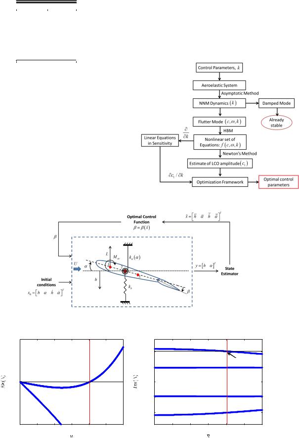
set of four first-order differential equations and represented in a statespace form. Varying u, a root locus plot can be used to compute the linear flutter velocity and frequency for the aeroelastic system. For the considered aeroelastic system with parameters shown in Table 1, the nondimensional linear flutter velocity is 0.807 and dimensionless linear flutter frequency is 0.1604. Figure 2 shows the locus of the real and imaginary part of the eigenvalue of the linearized aeroelastic system with respect to u.
III.Solution Approach
A strictly nonlinear state feedback control law is chosen with the coefficients of nonlinear terms considered as the control parameters. The control parameters are represented as a vector k. The asymptotic method [86] is used to compute the nonlinear normal modes for the closed-loop system dynamics. From the computed NNMs, the flutter
Downloaded by 94.180.100.60 on November 25, 2018 | http://arc.aiaa.org | DOI: 10.2514/1.C034239
SHUKLA AND PATIL |
1923 |
Table 1 Parameters used for airfoil section model
Parameter |
Value |
μ |
11 |
a |
−0.35 |
xα |
0.2 |
rα |
0.5 |
ω |
0.5 |
Gα |
0.5 |
T4 |
−0.4104 |
T10 |
1.6798 |
|
|
mode is identified and the fundamental harmonic balance method is used to obtain a set of algebraic nonlinear equations for the steadystate solution. For a fixed value of control parameters, these equations can be solved using Newton’s method to compute the LCO amplitude c1 and frequency ω. The set of equations is further differentiated with respect to each control parameter to obtain a set of linear equations for the sensitivities. The estimate of LCO amplitude and the corresponding analytical estimates of sensitivities are used to solve a multi-objective optimal control problem for the control parameters, which minimize the estimated LCO amplitude of flutter NNM and an approximate measure of the control cost. Figure 3 shows an outline of the solution approach. The accompanying sections describe the approach in detail.
IV. Nonlinear Normal Modes
Nonlinear normal modes extend the concept of linear normal modes to nonlinear systems. These were introduced in the 1960s by Rosenberg
[85,90,91] as the synchronous vibration of the system (i.e., all material points of the system reach their extreme values and pass through zero simultaneously, allowing all displacements to be expressed in terms of a single reference displacement). Shaw and Pierre [86,87,92] generalized Rosenberg’s definition of NNMs by defining them as two-dimensional invariant manifolds in phase space. An invariant set for a dynamic system is defined as a subset S of the phase space, such that starting from an initial condition in S the solution of governing equations of motions remains in S for all times. Moreover, this manifold can be parameterized
Fig. 3 Flowchart outlining the solution approach.
Fig. 1 Representation of two-dimensional airfoil section model. Points 1–3 represent the aerodynamic center, elastic axis location, and midchord point of the airfoil section.
0.05 |
|
|
|
|
|
|
|
|
|
|
|
|
|
|
|
|
|
|
1 |
Im(λ)=1.0080 |
|
|
|
|
|
|
|
|
|
|
|
|
|
|
|
|
|
|
|
|
|
|
|
|
0.5 |
|
|
|
|
ωf =1.0080/2π |
|
|
|
|
|
|
|
|
|
|
|
|
|
|
0 |
|
Re(λ)=0 |
|
|
|
0 |
|
|
UF =0.807 |
|
|
|
|
|
|
|
|
|
|
|
|
||||
|
|
|
|
UF =0.807 |
−0.5 |
|
|
|
|
|
|
|
|
|
|
|
|
|
|
|
|
|
|
||
|
|
|
|
|
|
−1 |
|
|
|
|
|
|
−0.05 |
0.2 |
0.4 |
0.6 |
0.8 |
1 |
0 |
0.2 |
0.4 |
0.6 |
0.8 |
1 |
1.2 |
0 |
||||||||||||
a) |
|
|
|
|
|
b) |
|
|
|
|
|
|
Fig. 2 Root locus plots of a) real part and b) imaginary part of eigenvalues with respect to the nondimensional velocity u.

Downloaded by 94.180.100.60 on November 25, 2018 | http://arc.aiaa.org | DOI: 10.2514/1.C034239
1924 |
SHUKLA AND PATIL |
in terms of a single pair of state variables (i.e., displacements and velocities of the chosen variable).
Shaw and Pierre’s approach has been applied for both continuous and discrete mechanical systems [86,87,92]. A short overview of computation of NNMs using the approach similar to Shaw and Pierre [86], as applied to the nonlinear aeroelastic system, is reviewed in this section. The nonlinear aeroelastic system’s governing equations of motion given in Eq. (1) can be represented in the form
2 h 3 |
2 x1 3 |
2 |
|
y1 |
|
|
3 |
|
|||
|
_ |
|
|
|
|
|
|
|
|
|
|
|
α |
7 |
x2 |
7 |
6 f1 |
|
y2 |
|
|
7 |
|
6 h |
6 y1 |
|
x1; x2; y1; y2 |
|
(4) |
||||||
6 |
|
7 |
6 |
7 |
6 |
|
|
|
|
7 |
|
6 |
α |
7 |
6 y2 |
7 |
6 f2 |
|
x1; x2; y1 |
; y2 |
|
7 |
|
4 |
|
5 |
4 |
5 |
4 |
|
|
5 |
|
||
where xi and yi represent the displacements and velocities, respectively, for the nondimensional plunge and pitch degrees of freedom. Pitch α is chosen as the master coordinate and the displacements and velocities in plunge are represented as nonlinear functions of the master coordinate:
x1 X1 u; v x2 u y1 Y1 u; v |
y2 v |
(5) |
where X1 u; v and Y1 u; v represent nonlinear |
functions |
of the |
master coordinates u and v. From Eq. (5), a normal mode can be defined as a motion taking place on a two-dimensional invariant manifold in the system’s phase space. This manifold passes through the equilibrium point of the system and is tangential to the eigenspace of the linear system, obtained by linearizing the nonlinear system about the equilibrium point. Differentiating Eq. (5) and using chain rule, we obtain
The nonlinear modal laws for the nonlinear system are approximated in the form of a polynomial in terms of the master coordinates up to the order equal to the degree of nonlinearity of the original equations of motion as
X1 u; v a1u a2v a3u2 a4uv a5v2 a6u3 a7u2v
a8uv2 a9v3 |
|
Y1 u; v b1u b2v b3u2 b4uv b5v2 b6u3 |
|
b7u2v b8uv2 b9v3 |
(9) |
Substituting Eq. (9) in Eq. (8), the coefficients of similar terms are collected and set to zero to obtain a set of nonlinear algebraic equations. Solving these equations, the coefficients (ai, bi) in the defined nonlinear modal laws become known and can be substituted into the equations corresponding to the master coordinate to obtain NNMs. The equations obtained by setting the coefficients to zero generally have multiple solutions, with each solution set corresponding to a different NNM. For the aeroelastic system, two sets of solutions are obtained. Defining a modal vector w u1 v1 u2 v2 T, a transformation can be defined from the modal coordinates to the physical coordinates z x1 x2 y1
z M w |
|
M0 M1 w M2 w w |
(10) |
where M0, M1, and M2 are defined as
|
|
|
2 a11 a21 a12 a22 3 |
|
|
|
|
2 a31u1 a41v1 |
a51v1 |
a32u2 a42v2 |
a52v2 3 |
||||||||||||||||||||||
|
M0 |
|
6 |
1 |
|
0 |
|
|
1 |
|
0 |
|
7; |
M1 |
w |
|
6 |
|
|
|
0 |
b41v1 |
|
0 |
|
b32u2 |
0 |
b42v2 |
0 |
7; and |
|||
|
|
6 b11 b21 b12 |
b22 |
7 |
|
|
|
6 b31u1 |
|
b51v1 |
|
b52v2 |
7 |
||||||||||||||||||||
|
|
|
6 |
|
|
|
|
|
|
|
|
|
7 |
|
|
|
|
6 |
|
|
|
|
|
|
|
|
|
|
|
7 |
|||
|
|
|
6 |
|
|
|
|
|
|
|
|
|
7 |
|
|
|
|
6 |
|
|
|
|
|
|
|
|
|
|
|
|
|
|
7 |
|
|
|
6 |
0 |
|
1 |
|
|
0 |
|
1 |
|
7 |
|
|
|
|
6 |
|
|
|
0 |
|
|
|
0 |
|
|
|
0 |
|
0 |
7 |
|
|
|
4 |
|
|
|
|
|
|
|
|
|
5 |
|
|
|
|
4 |
|
|
|
|
|
|
|
|
|
|
|
|
|
|
5 |
|
|
|
2 a61u12 a81v12 |
a71u12 a91v12 |
a62u22 a82v22 |
a72u22 a92v22 3 |
|
|
|
|
|||||||||||||||||||||||
M2 |
w |
|
6 |
|
|
0 |
b |
|
v2 |
b |
|
u2 |
0 |
b v2 |
b u2 |
0 |
b v2 |
b |
u2 |
0 |
b v2 |
7 |
|
|
|
|
|||||||
|
|
6 b u2 |
|
81 |
71 |
|
|
|
7 |
|
|
|
|
||||||||||||||||||||
|
|
|
6 |
61 |
1 |
|
|
1 |
|
|
1 |
|
91 |
1 |
62 |
2 |
|
82 |
2 |
|
72 |
2 |
|
92 |
2 |
7 |
|
|
|
|
|||
|
|
|
6 |
|
|
|
|
|
|
|
|
|
|
|
|
|
|
|
|
|
|
|
|
|
7 |
|
|
|
|
||||
|
|
|
6 |
|
|
0 |
|
|
|
|
|
|
|
0 |
|
|
|
|
0 |
|
|
|
|
|
|
0 |
|
|
7 |
|
|
|
|
|
|
|
4 |
|
|
|
|
|
|
|
|
|
|
|
|
|
|
|
|
|
|
|
|
|
|
|
|
|
5 |
|
|
|
|
x1 |
|
∂X1 |
u |
|
∂X1 |
v |
|
||
∂u |
|
∂v |
|
||||||
y1 |
|
∂Y1 |
u |
∂Y1 |
v |
(6) |
|||
∂u |
|
|
∂v |
|
|||||
From Eqs. (4) and (5), we obtain the following relations:
u v
v f2 X1 u; v ; u; Y1 u; v ; v |
(7) |
Substituting Eq. (7) in Eq. (6), the following relations are obtained:
Y |
|
|
u; v |
|
∂X1 u; v |
v |
|
∂X1 u; v |
f |
|
|
X |
|
|
u; v ; u; Y |
1 |
u; v ; v |
|||||||||||||||
|
1 |
|
|
|
|
|
∂u |
|
|
|
|
|
∂v |
|
|
|
2 |
1 |
|
|
||||||||||||
|
|
f |
|
|
X |
1 |
u; v ; u; Y |
1 |
u; v ; v |
∂Y1 u; v |
v |
|
|
|||||||||||||||||||
|
|
|
|
1 |
|
|
|
|
|
|
|
|
|
|
|
|
|
∂u |
|
|
|
|
|
|
||||||||
|
|
|
∂Y1 u; v |
f |
|
|
X |
1 |
u; v ; u; Y |
1 |
u; v |
; v |
|
|
|
(8) |
||||||||||||||||
|
|
|
|
∂v |
|
|
2 |
|
|
|
|
|
|
|
|
|
|
|
|
|
||||||||||||
where aij and bij represent the coefficients ai and bi in Eq. (9) for the jth NNM. Because the considered system has only cubic nonlinearity terms, M1 w 0. Assuming M−0 1M2 I, an approximate inverse transformation from physical to modal coordinates is defined as
w M w −1z |
|
M0 M2 w −1z |
|
I M0−1M2 w −1M0−1z |
|
I − M0−1M2 M0−1z M0−1z |
(11) |
The computed NNMs for the aeroelastic system with parameter values as given in Table 1 and at a velocity 1.05 times the nondimensional linear flutter velocity are stated next. The flutter NNM dynamics are given by
u1 u1 −1.00094 − 0.5541u12 0.005475u12 |
|
u1 0.004313 − 0.043356u12 − 0.03092u12 |
(12) |
Downloaded by 94.180.100.60 on November 25, 2018 | http://arc.aiaa.org | DOI: 10.2514/1.C034239
|
|
|
|
SHUKLA AND PATIL |
|
|
|
|
|
1925 |
|
0.1 |
|
|
|
|
0.1 |
|
|
|
|
|
|
0.05 |
|
|
|
|
0.05 |
|
|
|
|
|
|
0 |
|
|
|
|
0 |
|
|
|
|
|
|
−0.05 |
|
|
|
|
−0.05 |
|
|
|
|
|
|
−0.1 |
500 |
1000 |
1500 |
2000 |
−0.1 |
0 |
500 |
1000 |
1500 |
2000 |
2500 |
0 |
2500 |
||||||||||
0.4 |
|
|
|
|
0.4 |
|
|
|
|
|
|
0.2 |
|
|
|
|
0.2 |
|
|
|
|
|
|
0 |
|
|
|
|
0 |
|
|
|
|
|
|
−0.2 |
|
|
|
|
−0.2 |
|
|
|
|
|
|
−0.4 |
500 |
1000 |
1500 |
2000 |
−0.4 |
0 |
500 |
1000 |
1500 |
2000 |
2500 |
0 |
2500 |
||||||||||
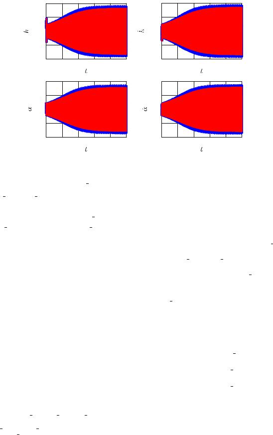
Fig. 4 Comparison of state responses obtained by simulating the complete aeroelastic system (dashed) and by transforming the modal response generated by simulation of NNM dynamics (solid).
A destabilizing linear damping term (0.004313u1) can be seen in Eq. (12) along with two stabilizing nonlinear damping terms (−0.043356u21u1 − 0.03092u31). The second NNM represents a damped oscillator for which the dynamics are given as
u2 u2 −0.23632 − 0.15194u22 2.2921u22 |
|
u2 −0.20603 1.1469u22 0.1142u22 |
(13) |
The stabilizing linear term is seen in Eq. (13). The process enables us to obtain completely decoupled NNMs represented in Eqs. (12) and (13) for the nonlinear aeroelastic system. Figure 4 compares the state response obtained by simulating the nonlinear aeroelastic system dynamics given in Eq. (4) and those obtained by transforming the modal response generated from the computed NNMs using the transformation defined in Eq. (10). Figure 4 also highlights the effectiveness of using NNM as a tool to capture the growth and amplitude of LCOs in aeroelastic systems.
V.Estimation of LCO Amplitudes
The harmonic balance method (HBM) is used to estimate the amplitude of the LCOs exhibited by the flutter NNM given in Eq. (12). The main idea behind HBM is to balance the Fourier components of dominant harmonics assuming the existence of a periodic limit cycle. HBM has been directly applied to aeroelastic systems to estimate LCO amplitudes in a number of works, such as Yang and Zhao [84], Liu and Dowell [93], and Dimitriadis [73]. In the current work, HBM is used to estimate the LCO amplitude of the flutter NNM.
A. Harmonic Balance Method
This section reviews the application of HBM for a second-order oscillator represented as
u f u; u fl u; u fnl u; u |
(14) |
where fl u; u and fnl u; u are strictly linear and |
nonlinear |
functions of u and u, respectively. It is assumed that the system exhibits a periodic response in steady state, which is approximated by a series of harmonic functions as
n |
|
|
up c0 Xk 1 |
ck cos kωt sk sin kωt |
(15) |
|
|
|
where c0 is a constant term, and ck and sk are coefficients of the cosine and sine terms of the kth harmonic, respectively. For n 1, the method is called the fundamental harmonic balance. Higher values of n correspond to higher order harmonic balance methods to get more accurate periodic solution approximations. The assumed solution is substituted back into the original system equations to obtain the following relation:
n
−ω2 Xk 1 k2 ci cos kωt si sin kωt f up; up |
|
|
|
fl up; up fnl up; up |
(16) |
The nonlinear function in Eq. (16), fnl up; up , is approximated as a summation of harmonics as shown here:
n |
|
fnl up; up cnl;0 Xk 1 |
cnl;k cos kωt snl;k sin kωt (17) |
|
|
where cnl;0, cnl;k, and snl;k can be computed in terms of previously
defined variables ω, c0, c1; : : : ; cn, and s1; : : : ; sn using the following integrals [73]:
|
ω |
2π∕ω |
|
|||
cnl;0 |
|
|
Z0 |
fnl up; up dt |
|
|
2π |
|
|||||
|
ω |
2π∕ω |
|
|
||
cnl;k |
|
Z0 |
|
fnl up; up cos kωt dt |
|
|
π |
|
|
||||
|
ω |
2π∕ω |
|
|
||
snl;k |
|
Z0 |
|
fnl up; up sin kωt dt |
(18) |
|
π |
|
|||||
Coefficients of constant term and sine and cosine terms of the same harmonics in Eq. (16) are collected and set to zero to obtain a set of nonlinear equations in the variables ω, c0, c1; : : : ; cn, and s2; : : : ; sn. For an autonomous system, s1 0 to avoid multiple solutions for the same LCO with different phase magnitudes. The obtained set of nonlinear equations can be solved using Newton’s method to compute the approximate periodic solution of the second-order oscillator. The number of harmonics considered determines the accuracy of the solution. In the current work, the fundamental harmonic balance method (n 1) is employed to compute the periodic solution of the flutter NNM.

Downloaded by 94.180.100.60 on November 25, 2018 | http://arc.aiaa.org | DOI: 10.2514/1.C034239
1926 |
SHUKLA AND PATIL |
B. Fundamental Harmonic Balance for LCO Nonlinear Normal Mode
The NNM exhibiting LCO at a nondimensional velocity of 1.05 times the linear flutter velocity is given in Eq. (12). The modal dynamics can be represented in the following shorthand form by
separating the linear terms in u and u: |
|
u p1u p2u fnl u; u |
(19) |
where p1 and p2 represent the coefficients of terms linear in u and u, respectively, whereas fnl u; u contains all the nonlinear terms of the LCO nonlinear normal mode. A periodic solution of the form given in Eq. (15) with n 1 is assumed:
u c0 c1 cos ωt |
(20) |
Using the assumed periodic solution, the first harmonic representation of the nonlinear terms in modal dynamics fnl u; u are obtained as shown in the previous section:
fnl u; u cnl;0 cnl;1 cos ωt snl;1 sin ωt |
(21) |
where cnl;0, cnl;1, and snl;1 can be computed in terms of c0, c1, and ω using Eq. (15). The periodic solution is substituted in the modal
dynamics (19) to obtain
−ω2c1 cos ωt p1 c0 c1 cos ωt p2ω −c1 sin ωt |
|
cnl;0 cnl;1 cos ωt snl;1 sin ωt |
(22) |
Collecting the constant, first harmonic sine and cosine terms in Eq. (22), we obtain a set of nonlinear algebraic equations:
p1c0 cnl;0 0 ω2c1 p1c1 cnl;1 0
(23)
− p2ωc1 snl;1 0
Because cnl;0, cnl;1, and snl;1 are nonlinear functions of c0, c1, and ω, Eq. (23) represents a set of three nonlinear algebraic equations that can be solved for the parameters c0, c1, and ω. The parameters c1 and ω represent the amplitude and frequency of the LCO exhibited by the flutter NNM with a static offset of c0.
VI. Closed-Loop System
To analyze the closed-loop system, a strictly nonlinear state feedback function is assumed as
|
3 |
|
3 |
_ 3 |
|
3 |
|
|
k2α |
|
|
k4α |
|
(24) |
|
β k1h |
|
k3h |
|
||||
where ki i 1; : : : ; 4 represents the control parameters. It is to be noted that linear control terms are not included because the focus of the present work is on nonlinear feedback control of LCO. Furthermore, a linear control law would be active over the entire range of operating conditions, whereas the nonlinear controller does not lead to significant actuation for low state response. Finally, a purely nonlinear controller also enables us to use the same linear modal solution while computing the nonlinear normal modes. The procedure of computation of NNMs shown in the preceding section is carried out for the closedloop system to obtain control-parameter-dependent nonlinear normal modal dynamics. The linear part of the computed NNMs remains unaltered, however, the nonlinear terms are now a function of the introduced control parameters ki i 1; 2; 3; 4 . The NNM corresponding to flutter mode can be represented in a general form as
u p1u p2u Fnl u; u; k |
(25) |
Having obtained the NNMs dependent on the control parameters, the fundamental harmonic balance method is used to obtain a set of three nonlinear equations, represented as
p1c0 cnl;0 c0; c1; ω; k1; k2; k3; k4 0
ω2c1 p1c1 cnl;1 c0; c1; ω; k1; k2; k3; k4 0 |
|
− p2ωc1 snl;1 c0; c1; ω; k1; k2; k3; k4 0 |
(26) |
It was stated earlier that the terms cnl;0, cnl;1, and snl;1 are nonlinear functions of c0, c1, and ω. For the closed-loop system, these terms will also be functions of the control parameters k1, k2, k3, and k4. For fixed values of control parameters, these equations can be solved using Newton’s method to compute c0, c1, and ω, which define the fundamental component of the periodic solution for the flutter mode NNM with amplitude c1, frequency ω, and static offset c0.
Differentiating Eq. (26) with respect to the control parameters, we obtain three sensitivity equations for each control parameter ki. These can be represented in the form of a linear matrix equation as
2 p1 |
∂c0 |
|
|
|
∂c1 |
|
|
|
|
|
|
|
|
∂ω |
|
|
|
|
|
38 |
∂ki |
9 |
||||||
|
|
|
∂cnl;0 |
|
|
|
∂cnl;0 |
|
|
|
|
|
|
∂cnl;0 |
|
|
> |
∂c0 |
> |
|||||||||
|
|
|
|
|
|
|
|
|
|
|
|
|
|
|
|
|
|
|
|
|
|
|
|
|
> |
|
|
> |
|
∂cnl;1 |
|
2 |
|
|
|
|
∂cnl;1 |
|
|
|
|
|
|
|
∂cnl;1 |
> |
∂c1 |
> |
|||||||||
6 |
|
|
|
|
|
|
p1 |
|
|
|
|
2ωc1 |
|
|
|
|
|
|
|
> |
|
|
> |
|||||
|
|
|
|
|
ω |
|
|
|
|
|
|
|
|
|
|
|
|
7> |
|
|
> |
|||||||
|
|
|
|
|
|
|
|
|
|
|
|
|
|
|
|
|
|
|
|
|
|
|
|
|
> |
|
|
> |
6 |
|
|
|
|
|
|
|
|
|
|
|
|
|
|
|
|
|
|
|
|
|
7> |
|
|
> |
|||
c |
|
|
|
|
|
c |
1 |
|
|
|
|
|
|
|
∂ |
ω |
k |
i |
||||||||||
6 |
∂ |
0 |
|
|
|
|
|
|
|
∂ |
|
|
|
|
|
|
|
|
|
|
|
7< |
∂ |
= |
||||
6 |
|
|
|
|
|
|
|
|
|
|
|
|
|
|
|
|
|
|
|
|
|
|
|
|
7 |
|
|
|
6 |
∂snl;1 |
|
− |
p |
ω ∂snl;1 |
− |
p |
c |
|
|
|
|
∂snl;1 |
7> |
∂ω |
> |
||||||||||||
|
|
|
|
|
1 |
|
|
|
|
|
|
|
|
|||||||||||||||
6 |
|
|
|
|
|
2 |
|
|
|
|
|
2 |
|
|
|
|
|
|
|
|
7> |
|
|
> |
||||
4 |
∂c0 |
|
|
|
|
∂c1 |
|
|
|
|
|
|
|
∂ω |
> |
∂ki |
> |
|||||||||||
|
|
|
|
|
|
|
|
|
|
|
5> |
> |
||||||||||||||||
|
|
|
|
|
|
|
|
|
|
|
|
|
|
|
|
|
|
|
|
|
|
|
|
|
> |
|
|
> |
|
|
|
|
|
|
|
|
|
|
|
|
|
|
|
|
|
|
|
|
|
|
|
|
|
> |
|
|
> |
|
|
|
|
|
|
|
|
|
|
|
|
|
|
|
|
|
|
|
|
|
|
|
|
|
> |
|
|
> |
|
|
8 |
∂cnl;0 |
9 |
|
|
|
|
|
|
|
|
|
|
|
|
|
|
|
|
|
|
: |
|
|
; |
||
|
|
∂ki |
|
|
|
|
|
|
|
|
|
|
|
|
|
|
|
|
|
|
|
|
|
|
||||
|
|
> |
|
|
> |
|
|
|
|
|
|
|
|
|
|
|
|
|
|
|
|
|
|
|
|
|
|
|
|
|
> |
|
|
> |
|
|
|
|
|
|
|
|
|
|
|
|
|
|
|
|
|
|
|
|
|
|
|
|
|
> |
∂cnl;1 |
> |
|
|
|
|
|
|
|
|
|
|
|
|
|
|
|
|
|
|
|
|
|
|
||
|
−> |
|
|
> |
|
|
|
|
|
|
|
|
|
|
|
|
|
|
|
|
|
|
|
|
|
(27) |
||
|
|
> |
|
|
> |
|
|
|
|
|
|
|
|
|
|
|
|
|
|
|
|
|
|
|
|
|
||
|
|
> |
|
|
> |
|
|
|
|
|
|
|
|
|
|
|
|
|
|
|
|
|
|
|
|
|
|
|
|
|
> |
k |
|
> |
|
|
|
|
|
|
|
|
|
|
|
|
|
|
|
|
|
|
|
|
|
|
|
|
|
< |
∂ |
i |
= |
|
|
|
|
|
|
|
|
|
|
|
|
|
|
|
|
|
|
|
|
|
|
|
|
|
> |
∂snl;1 |
> |
|
|
|
|
|
|
|
|
|
|
|
|
|
|
|
|
|
|
|
|
|
|
||
|
|
> |
|
|
> |
|
|
|
|
|
|
|
|
|
|
|
|
|
|
|
|
|
|
|
|
|
|
|
|
|
> |
∂ki |
> |
|
|
|
|
|
|
|
|
|
|
|
|
|
|
|
|
|
|
|
|
|
|
||
|
|
> |
> |
|
|
|
|
|
|
|
|
|
|
|
|
|
|
|
|
|
|
|
|
|
|
|||
|
|
> |
|
|
> |
|
|
|
|
|
|
|
|
|
|
|
|
|
|
|
|
|
|
|
|
|
|
|
|
|
> |
|
|
> |
|
|
|
|
|
|
|
|
|
|
|
|
|
|
|
|
|
|
|
|
|
|
|
|
|
> |
|
|
> |
|
|
|
|
|
|
|
|
|
|
|
|
|
|
|
|
|
|
|
|
|
|
|
|
|
: |
|
|
; |
|
|
|
|
|
|
|
|
|
|
|
|
|
|
|
|
|
|
|
|
|
|
|
The preceding equation can be solved using linear solvers to generate analytical estimates of sensitivities. The sensitivity of response variables with respect to the control parameter ki can be represented by ∂ : ∕∂ki . The computed analytical sensitivities of c1 with respect to the control parameters ∂c1∕∂ki for i 1; : : : ; 4 are used for control design.
The estimate of LCO amplitude c1 uses NNM and HBM to approximate the amplitude of the flutter NNM. To validate the approach, the analytical sensitivities of the estimated LCO amplitude ∂c1∕∂ki are compared with the numerically computed sensitivities of the LCO amplitude calculated from simulation of the complete nonlinear aeroelastic system and the flutter NNM. The numerical sensitivities are computed by employing finite difference on the LCO amplitudes, estimated from the steady-state time response of the NNM dynamics and the complete system dynamics:
A |
|
A ki ki − A ki |
(28) |
|
ki |
||||
ki |
|
where A represents the LCO amplitude. A can be estimated numerically by simulating the flutter mode NNM dynamics or the complete nonlinear aeroelastic system using Runge–Kutta method.
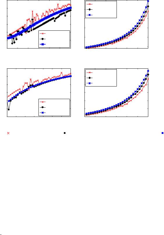
Figure 5 compares the sensitivities of LCO exhibited by flutter NNM with respect to the control parameters ki obtained using the finite difference method A∕ ki and the analytical estimates ∂c1∕∂ki obtained using Eq. (27). The finite difference method to compute sensitivities involves numerical estimation of the amplitude of flutter NNM followed by application of finite difference on the estimated amplitude, making it prone to machine precision errors, as seen in the figures. Moreover, it becomes computationally expensive if used in an optimization problem that requires the sensitivities at each step. From Fig. 5, it is clear that analytical estimates of sensitivities obtained by the harmonic balance method match closely with the finite difference sensitivities obtained on numerically estimated amplitudes. The next section describes a multi-objective optimization framework that uses the estimated analytical sensitivities at each step.
Downloaded by 94.180.100.60 on November 25, 2018 | http://arc.aiaa.org | DOI: 10.2514/1.C034239
SHUKLA AND PATIL |
1927 |
−2 x 10⁻⁴ |
|
|
|
|
|
|
6 |
x 10−3 |
|
|
|
|
|
||
−3 |
|
|
|
|
|
|
|
|
|
A / |
k2 −NNM |
|
|
|
|
|
|
|
|
|
|
|
5 |
|
A/ |
k −Full |
|
|
|
||
|
|
|
|
|
|
|
|
|
|
|
2 |
|
|
|
|
−4 |
|
|
|
|
|
|
|
4 |
|
∂ c1/∂ k2 |
|
|
|
|
|
|
|
|
|
|
|
|
|
|
|
|
|
|
|
|
|
−5 |
|
|
|
|
|
|
|
|
|
|
|
|
|
|
|
|
|
|
|
|
|
|
|
3 |
|
|
|
|
|
|
|
−6 |
|
|
|
|
A / |
k1 −NNM |
|
|
|
|
|
|
|
|
|
|
|
|
|
|
2 |
|
|
|
|
|
|
|
|||
−7 |
|
|
|
|
A/ |
k1 −Full |
|
|
|
|
|
|
|
|
|
|
|
|
|
|
|
|
|
|
|
|
|
|
|||
−8 |
|
|
|
|
∂ c1/∂ k1 |
|
1 |
|
|
|
|
|
|
|
|
|
|
|
|
|
|
|
|
|
|
|
|
|
|
||
−50 |
0 |
|
50 |
100 |
150 |
200 |
−40 |
−35 |
−30 |
−25 |
−20 |
−15 |
−10 |
||
−100 |
|
||||||||||||||
a) |
|
|
|
k1 |
|
|
|
b) |
|
|
|
k2 |
|
|
|
|
|
|
|
|
|
|
|
|
|
|
|
|
|
||
−0.5 x 10⁻³ |
|
|
|
|
|
|
7 |
x 10−3 |
|
|
|
|
|
||
−1 |
|
|
|
|
|
|
|
6 |
|
A / |
k4 −NNM |
|
|
|
|
|
|
|
|
|
|
|
|
A/ |
k4 −Full |
|
|
|
|||
|
|
|
|
|
|
|
|
|
|
|
|
|
|||
−1.5 |
|
|
|
|
|
|
|
5 |
|
∂ c1/∂ k4 |
|
|
|
|
|
−2 |
|
|
|
|
|
|
|
4 |
|
|
|
|
|
|
|
−2.5 |
|
|
|
|
A / |
k3 −NNM |
3 |
|
|
|
|
|
|
|
|
|
|
|
|
|
|
|
|
|
|
|
|
|
|||
−3 |
|
|
|
|
A/ |
k3 −Full |
|
2 |
|
|
|
|
|
|
|
−3.5 |
|
|
|
|
∂ c1/∂ k3 |
|
1 |
|
|
|
|
|
|
|
|
−10 |
0 |
10 |
20 |
30 |
40 |
50 |
|
−35 |
−30 |
−25 |
−20 |
−15 |
−10 |
||
−20 |
−40 |
||||||||||||||
c) |
|
|
|
k3 |
|
|
|
d) |
|
|
|
k4 |
|
|
|
Fig. 5 Comparison of numerical sensitivities A∕ ki obtained by applying finite difference on amplitudes estimated from time simulation of flutter mode NNM dynamics ( ), complete aeroelastic system dynamics ( ), and approximate analytical sensitivities ∂c1∕∂ki obtained using HBM ( ) while varying a) k1, b) k2, c) k3, and d) k4.
VII. Optimization Framework
The objective of optimization problem is to find optimal control parameters that minimize the LCO amplitude of the nonlinear aeroelastic system and the control cost. The problem is formulated as a weighted sum multi-objective optimization with the two objectives. The estimate of LCO amplitude of the flutter NNM (i.e., c1) is used
along with an approximate measure of the control cost ccapprox described next. It is subsequently shown that reducing c1 ends up in
reduction of the LCO amplitude of the complete aeroelastic system by approximately the same percentage.
A. Approximate Control Cost
The measure of approximate control cost used involves considering the linear flutter mode at the linear flutter velocity. The
eigenvector corresponding |
to |
the linear |
flutter mode at UF |
|||||||||
|
|
|
|
|
|
|
|
|
|
|
|
|
normalized with respect to the h coordinate is stated as |
|
|||||||||||
2 |
|
3 |
|
|
|
2 |
|
λr |
1 |
iλi |
3 |
|
α |
|
|
|
|
|
|||||||
|
h |
7 |
|
|
6 |
|
|
|
7 |
|
||
6 h |
iγi |
|
iωf |
|
||||||||
6 |
_ |
7 |
γr |
|
6 |
|
λr |
|
λi iωf |
7 |
(29) |
|
α |
|
|
|
|
|
|
||||||
4 |
|
5 |
|
|
|
4 |
|
|
|
|
5 |
|
Based on the normalized linear flutter modes, the amplitudes of the state variables can be approximated as
|
2 |
1 |
3 |
|
2 |
|
1 |
|
λi2 |
|
3 |
|
||
|
α0 |
|
|
λr2 |
|
|
|
|
||||||
|
6 |
ωf |
7 |
q6 |
p |
|
7 |
|
||||||
ho |
|
|
|
γr2 |
γi2 |
|
|
|
|
|
|
|
(30) |
|
|
6 |
|
7 |
|
6 |
|
ω |
|
|
|
|
7 |
|
|
|
α0ωf |
|
ω |
λ2 |
|
λ2 |
|
|||||||
|
4 |
|
5 |
|
4 |
f |
|
r |
|
i |
5 |
|
||
|
|
|
|
|
|
|
p |
|
|
|||||
For the considered system, the parameters α0 and ωf are 3.7645 and 1.0085, respectively. The approximate control cost is defined as
ccapprox fkgT Qfkg |
(31) |
where Q 1; α60; ω6f; α0ωf 6 R4×4 is a diagonal matrix, with the diagonal terms representing the expected effect of the coefficients in
the cubic control law.
B. Optimization Problem
The optimization problem is represented as
|
|
min |
λc |
|
k |
|
1 |
− |
λ cc |
k |
|
|
|
k |
1 |
|
|
|
approx |
(32) |
|||
|
|
subject to |
lb ≤ k ≤ ub |
|
|
|
|
||||
where |
k |
represents |
the |
|
vector |
|
of |
control |
parameters |
||
k k1 |
k2 |
k3 k4 T ; lb and ub represent the lower and upper |
|||||||||
bounds on the control parameter vector, respectively; and λ is a weight parameter that can be chosen depending on the desired amount of control, from low authority (λ 0) to high authority (λ 1). The control vector k needs to be bounded to guarantee physically relevant response of both the aeroelastic system and the NNMs. These bounds can be computed by guaranteeing that the overall nonlinear stiffness always remains positive, subject to the different values of the state variables. In the case of multiple nonlinearities, the corresponding eigenvalues of the overall nonlinear stiffness matrix should always remain positive for different values of statevariables. In the current work, numerical simulations are conducted to identify these bounds based on the response of the aeroelastic system and the NNM dynamics. These bounds are not related to any physical actuator constraints.
Downloaded by 94.180.100.60 on November 25, 2018 | http://arc.aiaa.org | DOI: 10.2514/1.C034239
1928 |
SHUKLA AND PATIL |
For a fixed value of k, both c1 and ccapprox and the corresponding sensitivities can be computed by solving the HBM equations given in Eq. (26) using Newton’s method and Eq. (27) using a linear solver respectively. The solution of the optimization problem for a given value of the weighing parameter λ 0; 1 is represented by kopt λ . Choosing the lower and upper bounds as
lb −230 −230 −60.0 −230 T ; ub 230 1 230 5 T
(33)
the sequential quadratic programming algorithm in MATLAB is used to solve the optimization problem, using the analytically generated sensitivities. The cost functions in the multi-objective optimization problem are scaled to obtain the following problem:
|
|
k |
c1 |
kopt λ 0 |
|
− |
|
ccapprox kopt λ 1 |
(34) |
||
|
min |
λ |
c1 k |
|
1 |
|
λ |
|
ccapprox k |
|
|
subject to |
|
|
lb ≤ k ≤ ub |
|
|
||||||
(normalized) |
|
1 |
λ=1 |
|
|
|
|
|
|
|
|
|
0.8 |
|
|
|
|
|
|
|
|
|
|
|
|
|
|
|
|
|
|
|
|
|
|
|
|
0.6 |
|
|
|
|
|
|
|
|
|
approx |
0.4 |
|
|
|
|
|
|
|
|
|
|
|
|
|
|
|
|
|
|
|
|
|
|
cc |
|
0.2 |
|
|
|
|
|
|
|
|
|
|
|
|
|
|
|
|
|
|
|
|
|
|
|
0 |
|
|
|
|
|
|
|
λ=0 |
|
|
|
|
0.2 |
0.4 |
|
|
0.6 |
0.8 |
1 |
||
|
|
0 |
|
|
|
||||||
c1 (normalized)
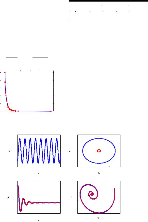
Fig. 6 Pareto front obtained using weighted sum multi-objective optimization approach.
0.4
0.2
0


−0.2
−0.4 


 3950 3960 3970 3980 3990 4000
0.02
0.01
0
−0.01
0 |
50 |
100 |
Table 2 Comparison of LCO amplitudes for openand closed-loop response of flutter NNM dynamics
|
Open loop |
|
Closed loop |
|
||
|
|
|
|
|
|
% reduction in |
State |
Amplitude |
Frequency |
|
Amplitude |
Frequency |
amplitude |
u1 |
0.3042 |
1.0195 |
0.02822 |
1.0007 |
90.72 |
|
v1 |
0.3082 |
1.0195 |
0.02824 |
1.0007 |
90.83 |
|
|
|
|
|
|
|
|
Solving the optimization problem with the scaled cost functions for varying values of λ, a set of optimal controllers can be generated.
VIII. Results
Depending on the requirements on the amplitude of LCO, λ can be chosen between zero and one to obtain the corresponding optimal control parameters. Using λ 1 will result in parameters that minimize the amplitude of LCO NNM, whereas λ 0 minimizes only the approximate control cost and will lead to no control. Figure 6 shows the variations of the normalized cost functions for varying values of λ 0; 1 . It is seen that increasing λ results in decrease of c1
and an increase of ccapprox. Both the normalized costs have a maximum value of one because of the scaling factors used.
To minimize the LCO amplitude, λ close to one is chosen. For λ 0.97, the optimal control parameters obtained are
kopt λ 0.97 2.86 −201.42 9.13 −63.60 T |
(35) |
The periodic solution obtained from the harmonic balance
equations for the open- k 0 and closed-loop k kopt cases are stated as
ω |
|
|
1.0254 |
; |
ω |
|
|
1.0007 |
|
(36) |
c1 |
|
|
0.3499 |
|
c1 |
|
|
0.0337 |
|
|
|
k 0 |
|
|
|
|
k kopt |
|
|
|
|
The percentage decrease in c1 from the opento the closed-loop case comes out to be 90.369%.
0.4
0.2
0
−0.2
−0.4 |
−0.2 |
0 |
0.2 |
0.4 |
−0.4 |
||||
4 x 10⁻³ |
|
|
|
|
2 |
|
|
|
|
0 |
|
|
|
|
−2 |
|
|
|
|
−4 |
|
|
|
|
−6 |
0 |
|
0.01 |
0.02 |
−0.01 |
|
Fig. 7 Comparison of the open-loop k 0 |
(dashed |
line) and the closed-loop k |
|
k (solid line) response of the NNM dynamics, subject to the initial |
||||
|
T |
|
|
|
opt |
|||
conditions w0 −0.0140 −0.0181 0.0240 0.0181 |
|
; (u1 |
, v1) and (u2 |
, v2) are the flutter mode and damped mode states, respectively. |
||||
Downloaded by 94.180.100.60 on November 25, 2018 | http://arc.aiaa.org | DOI: 10.2514/1.C034239
|
|
|
|
|
SHUKLA AND PATIL |
|
|
|
1929 |
|||
0.1 |
|
|
|
|
|
|
0.1 |
|
|
|
|
|
0.05 |
|
|
|
|
|
|
0.05 |
|
|
|
|
|
¯ h |
0 |
|
|
|
|
|
¯ h |
0 |
|
|
|
|
|
|
|
|
|
|
|
˙ |
|
|
|
|
|
−0.05 |
|
|
|
|
|
−0.05 |
|
|
|
|
||
−0.1 |
|
1000 |
2000 |
|
3000 |
−0.1 |
−0.05 |
0 |
0.05 |
0.1 |
||
|
0 |
|
|
−0.1 |
||||||||
|
|
|
|
|
t |
|
|
|
|
¯ |
|
|
|
|
|
|
|
|
|
|
|
|
h |
|
|
0.4 |
|
|
|
|
|
|
0.4 |
|
|
|
|
|
0.2 |
|
|
|
|
|
|
0.2 |
|
|
|
|
|
α |
0 |
|
|
|
|
|
α˙ |
0 |
|
|
|
|
−0.2 |
|
|
|
|
|
|
−0.2 |
|
|
|
|
|
−0.4 |
|
1000 |
2000 |
|
3000 |
−0.4 |
−0.2 |
0 |
0.2 |
0.4 |
||
|
0 |
|
|
−0.4 |
||||||||
|
|
|
|
|
t |
|
|
|
|
α |
|
|
Fig. 8 Comparison of open-loop k 0 |
(dashed) and closed-loop k |
|
k (solid) state response and phase-plane plot for the aeroelastic system, subject to |
|||||||||
0 |
T |
|
|
opt |
|
|
|
|
|
|||
initial conditions z0 0.01 |
0.1 0 |
|
. |
|
|
|
|
|
|
|
|
|
A. NNM Response |
|
The open- k 0 and closed-loop k kopt NNM dynamics are |
|
simulated subject |
Tto initial conditions w0 −0.084 |
−0.00170.01570.0017 |
. Figure 7 compares the openand closed- |
loop time response and phase-plane plots of the NNM dynamics. It is seen that the flutter NNM exhibits LCOs, whereas the damped mode attains the equilibrium state. The amplitude of LCO in the closed-loop case is clearly much smaller than that of the open-loop case, as seen in the phase-plane plots.
Table 2 compares the numerically estimated amplitudes for the LCO exhibited by flutter NNM. It can be seen that the closed-loop LCO amplitude is around 90% less than that of the open-loop LCO amplitude. This is very close to the percentage decrease observed in c1 between the openand closed-loop cases.
B. Nonlinear Aeroelastic System Response
The open- k 0 and closed-loop k kopt nonlinear aeroelastic
system dynamics are |
simulated subject to initial conditions x |
0 |
|
||
|
T |
|
|||
0.01 0 0.1 0 0 |
|
as shown in Fig. 8, which compares the |
|||
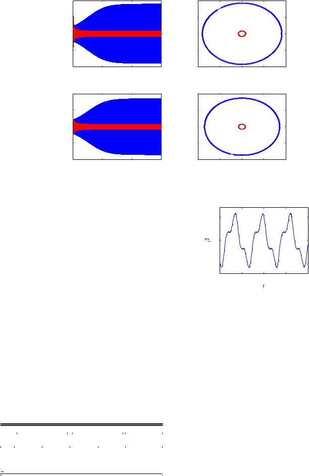
time response as well as the phase-plane plots. It can be seen that the system states are executing LCOs for both the openand closed-loop cases, however, the amplitude of LCO is much less for the closedloop response. This is expected because the optimal controller used for the closed-loop case corresponds to λ 0.97. The reduction in LCO amplitude can be seen more clearly in the phase-plane plots for pitch and nondimensional plunge degree of freedom, shown in Fig. 8.
Table 3 compares the numerically estimated LCO amplitudes for pitch and nondimensional plunge degree of freedom for openand
Table 3 Comparison of LCO amplitudes in pitch and nondimensional plunge degrees of freedom of the nonlinear aeroelastic system for openand closed-loop cases
|
Open loop |
|
Closed loop |
|
|
||
|
|
|
|
|
|
|
% reduction in |
State |
Amplitude |
Frequency |
|
Amplitude |
Frequency |
|
amplitude |
|
0.0903 |
1.0245 |
0.00829 |
1.0007 |
90.82 |
||
h |
|||||||
α |
0.3414 |
1.0243 |
0.0304 |
1.0007 |
91.08 |
||
_ |
|
|
|
|
|
|
|
|
0.0930 |
1.0245 |
0.00832 |
1.0007 |
91.04 |
||
h |
|||||||
α |
0.3470 |
1.0245 |
0.0305 |
1.0007 |
91.22 |
||
|
|
|
|
|
|
|
|
|
|
|
|
|
|
|
|
x 10−3
5
0
−5
3980 3985 3990 3995 4000
Fig. 9 Generated periodic control input using the nonlinear feedback control function with the control parameter vector k kopt.
closed-loop case. The LCO amplitudes for the closed-loop case are around 91% less than the LCO amplitudes in the open-loop case. This is quite close to the percentage decrease in the numerically estimated LCO amplitude of flutter NNM and LCO amplitude estimate of flutter NNM obtained from HBM c1. It can be concluded that minimizing c1 results in reduction of LCO amplitudes exhibited by the flutter NNM and the complete aeroelastic system states by approximately the same amount.
Using the time response of the displacements and velocities in pitch and nondimensional plunge degree of freedom, the nonlinear feedback control input signal can be computed. The control input for a section of simulation time when the aeroelastic system states are executing LCOs is shown in Fig. 9. It can be seen that, after the system states start exhibiting LCOs, the nonlinear control input is essentially a periodic signal with its maximum absolute value being 5.7 × 10⁻³ rad for the control parameter vector k kopt.
C. Effect of Nonzero Acceleration
A nonzero acceleration will result in a changing freestream velocity for the aeroelastic system. Hence, the assumption that the linear terms of the considered aeroelastic system remains the same will not be valid. A constant freestream velocity of 1.05Uf was considered to derive the controller and the simulation results in the preceding section. In the current section, a simulation-based study is
Downloaded by 94.180.100.60 on November 25, 2018 | http://arc.aiaa.org | DOI: 10.2514/1.C034239
1930 |
SHUKLA AND PATIL |
inreduction“%LCO amplitude |
80 |
|
|
|
|
βofAmplitude(rad) |
0.01 |
|
100 |
|
|
|
|
α |
0.05 |
|
95 |
|
|
|
|
h |
0.04 |
|
90 |
|
|
|
|
|
0.03 |
|
85 |
|
|
|
|
|
0.02 |
10a to |
75 |
1.05 |
1.1 |
1.15 |
1.2 |
1.25 |
0 |
|
1 |
1 |
|||||
a) |
|
|
|
U/Uf |
|
b) |
|
1.05 |
1.1 |
1.15 |
1.2 |
1.25 |
U/Uf
Fig. 10 Effect of varying velocity on performance of the controller formulated at U 1.05Uf : a) Percentage reduction in LCO amplitude of closed-loop response; b) amplitude of control input β when the closed-loop response settles in LCO.
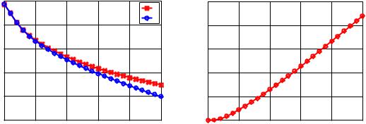
carried out to study the performance of the developed controller at changing velocities. The controller formulated at a velocity of U 1.05Uf is used to generate the closed-loop response of the aeroelastic system at different velocities.
From Fig. 10, it is clear that the controller formulated at U 1.05Uf successfully reduces the LCO amplitude at other velocities. However, the percentage reduction in amplitude at higher velocities slightly decreases from 90% at 1.05 Uf to 80% at 1.25 Uf. Furthermore, there is a tenfold increase in the control requirements. The increase in control requirements is expected with an increase in the energetics of the instability, though some of the increase can also be attributed to the fact that the controller is not optimal for the other velocities. To further optimize the controller, depending on the requirements, a bank of controllers can be formulated beforehand and scheduled with respect to the velocity.
IX. Conclusions
A methodology to compute analytical estimates of LCO amplitudes and its sensitivities to the introduced control parameters is developed for a nonlinear aeroelastic system. The process involves the computation of nonlinear normal modes and use of the harmonic balance method. The analytical estimates of sensitivity are shown to be consistent with the numerically generated sensitivities using the finite difference method. This is quite useful because the sensitivities obtained using finite difference are prone to machine precision errors and requires a lot of computational effort for large-scale systems. The analytical estimates of sensitivities are used to solve a multi-objective optimization problem that generates optimal control parameters to minimize LCO amplitudes of the flutter nonlinear normal mode (NNM). Numerical simulations are used to verify that minimizing the estimated analytical LCO amplitude of flutter NNM corresponds directly to minimizing the LCO amplitude of the aeroelastic system. Higher order harmonic balance methods can be used to come up with a more accurate prediction of the periodic solution, thereby giving more accurate estimates of LCO amplitude and their corresponding sensitivities.
References
[1]Raghothama, A., and Narayanan, S., “Non-Linear Dynamics of a TwoDimensional Airfoil by Incremental Harmonic Balance Method,” Journal of Sound and Vibration, Vol. 226, No. 3, 1999, pp. 493–517. doi:10.1006/jsvi.1999.2260
[2]Liu, L., Wong, Y. S., and Lee, B. H. K., “Application of the Centre Manifold Theory in Non-Linear Aeroelasticity,” Journal of Sound and Vibration, Vol. 234, No. 4, 2000, pp. 641–659. doi:10.1006/jsvi.1999.2895
[3]Dowell, E. H., and Tang, D., “Nonlinear Aeroelasticity and Unsteady Aerodynamics,” AIAA Journal, Vol. 40, No. 9, 2002, pp. 1697–1707. doi:10.2514/2.1853
[4]Lee, B. H. K., Price, S. J., and Wong, Y. S., “Nonlinear Aeroelastic Analysis of Airfoils: Bifurcation and Chaos,” Progress in Aerospace Sciences, Vol. 35, No. 3, 1999, pp. 205–334. doi:10.1016/S0376-0421(98)00015-3
[5]Gilliatt, H. C., Strganac, T. W., and Kurdila, A. J., “An Investigation of Internal Resonance in Aeroelastic Systems,” Nonlinear Dynamics, Vol. 31, No. 1, 2003, pp. 1–22.
doi:10.1023/A:1022174909705
[6]Woolston, D. S., Runyan, H. L., and Byrdsong, T. A., “Some Effects of System Nonlinearities in the Problem of Aircraft Flutter,” NACA Technical Rept. 3539, 1955.
[7]Woolston, D. S., “An Investigation of Effects of Certain Types of Structural Nonlinearities on Wing and Control Surface Flutter,” Journal of the Aeronautical Sciences, Vol. 24, No. 1, 1957, pp. 57–63.
[8]Shen, S. F., “An Approximate Analysis of Nonlinear Flutter Problems,”
Journal of the Aerospace Sciences, Vol. 26, No. 1, 1959, pp. 25–32.
[9]Breitbach, E., “Effects of Structural Non-Linearities on Aircraft Vibration and Flutter,” Defense Technical Information Center Doc., AGARD Technical Rept. 665, 1978.
[10]Breitbach, E. J., “Flutter Analysis of an Airplane with Multiple Structural Nonlinearities in the Control System,” NASATechnical Rept. 1620, 1980.
[11]Thompson, D. E., and Strganac, T. W., “Store-Induced Limit Cycle Oscillations and Internal Resonances in Aeroelastic Systems,” AIAA Paper 2000-1413, 2000.
[12]Sheta, E. F., Harrand, V. J., Thompson, D. E., and Strganac, T. W., “Computational and Experimental Investigation of Limit Cycle Oscillations of Nonlinear Aeroelastic Systems,” Journal of Aircraft, Vol. 39, No. 1, 2002, pp. 133–141.
doi:10.2514/2.2907
[13]Denegri, C. M., “Limit Cycle Oscillation Flight Test Results of a Fighter with External Stores,” Journal of Aircraft, Vol. 37, No. 5, 2000, pp. 761–769.
doi:10.2514/2.2696
[14]Trame, L. W., Williams, L. E., and Yurkovich, R. N., “Active Aeroelastic Oscillation Control on the F/A-18 Aircraft,” AIAA, New York, 1985, pp. 19–21; also AIAA Paper 1985-1858, 1985.
[15]Noor, A. K., and Venneri, S. L., “Flight-Vehicle Materials, Structures, and Dynamics-Assessment and Future Directions,” Vol. 5, Structural Dynamics and Aeroelasticity, American Soc. of Mechanical Engineers, New York, 1993, pp. 179–212.
[16]Lyons, M. G., Vepa, R., Mcintosh, S. C., Jr., and DeBra, D. B., “Control Law Synthesis and Sensor Design for Active Flutter Suppression,” AIAA Paper 1973-832, 1973.
[17]Mukhopadhyay, V., Newsom, J. R., and Abel, I., “A Direct Method for Synthesizing Low-Order Optimal Feedback Control Laws with Application to Flutter Suppression,” Proceedings of the AIAA Atmospheric Flight Mechanics Conference, AIAA, New York, 1980, pp. 465–475.
[18]Gangsaas, D., Ly, U., and Norman, D. C., “Practical Gust Load Alleviation and Flutter Suppression Control Laws Based on a LQG Methodology,” 19th Aerospace Sciences Meeting, AIAA Paper 19810021, Jan. 1981, p. 11 (in English).
[19]Karpel, M., “Design for Active Flutter Suppression and Gust Alleviation Using State-Space Aeroelastic Modeling,” Journal of Aircraft, Vol. 19, No. 3, 1982, pp. 221–227.
doi:10.2514/3.57379