1_c033999

I.Introduction

THE next generation of military and commercial rotorcraft is expected to reach substantially higher speeds than platforms currently in production through the use of advanced configurations. One possible configuration is a coaxial helicopter with thrust and/or lift compounding, obtained through the addition of pusher propellers and/or wings. To fully leverage the benefits provided by these configurations, improved analysis and design methodologies will be

required.

The present paper explores the use of formal numerical optimization methodologies in rotorcraft preliminary design. Although such methodologies have existed for decades, their use in preliminary design of rotorcraft has been rather limited, as pointed out by surveys such as [1,2].

In a more recent comprehensive report [3], Orr and Narducci addressed “current” (as of 2008) and potential uses of optimization

Received 10 May 2016; revision received 19 October 2016; accepted for publication 7 November 2016; published online Open Access 7 April 2017. Copyright © 2016 by the authors. Published by the American Institute of Aeronautics and Astronautics, Inc., with permission. All requests for copying and permission to reprint should be submitted to CCC at www.copyright.com; employ the ISSN 0021-8669 (print) or 1533-3868 (online) to initiate your request. See also AIAA Rights and Permissions www.aiaa.org/randp.

*Doctoral Candidate, Alfred Gessow Rotorcraft Center, Department of Aerospace Engineering; shersey@umd.edu.

†Research Associate, Alfred Gessow Rotorcraft Center, Department of Aerospace Engineering; ananth@umd.edu.

‡Professor, Alfred Gessow Rotorcraft Center, Department of Aerospace Engineering; celi@umd.edu.

by the helicopter industry, with special focus on the use of highfidelity analysis tools and multidisciplinary design optimization [3]. Most optimization occurred in disciplinary areas such as rotor aerodynamics, rotor structures and dynamics, fuselage aerodynamics and structures, and propulsion and drive systems. Conceptual and preliminary designs were based on sizing codes that use low-fidelity analysis methods, although moving high-fidelity analyses into conceptual design was an emerging trend. From [3], “[Preliminary design] is when multi-disciplinary optimization with high-fidelity analysis can benefit design and needs to be developed for the rotorcraft industry. Optimization should be targeted toward an early phase of design, when the majority of life cycle cost is determined.”

An example of the point of view of rotorcraft government laboratories, which require design capabilities to support research and acquisition but do not typically build actual aircraft, was presented by Johnson and Sinsay [4]. Conceptual design was again based primarily on low-fidelity tools. The primary role of high-fidelity analyses was to support development and calibration of low-fidelity models. Between a “high-fidelity” analysis and a “low-fidelity” analysis, a “right-fidelity” analysis was defined, as “the minimum level of fidelity needed to reach an acceptable level of uncertainty” [5]. Optimization was given primarily a local, rather than a system, role. This philosophy was embodied in recent studies such as the performance design exercises on heavy-lift rotorcraft configurations [6], slowed-rotor tandem compounds [7], coaxial compounds [8], and cruise-efficient single-main rotor compounds [9].

The use of formal numerical optimization techniques in conceptual and preliminary design can yield significant benefits. First, the optimizer automatically takes into account all interactions among all design parameters and across all disciplines included in the analysis model. Second, the optimizer has no subjective bias and will select the best design(s), possibly including some apparently counterintuitive ones. Third, the solution will indicate what constraints limit further design improvements and quantify design tradeoffs through multiobjective formulations or sensitivity analyses. Finally, once objective(s) and constraints are properly formulated, with proper software logic implemented, most of the intermediate portions of the design process can be left to the computer, with little or no analyst involvement.

From a numerical optimization viewpoint, conceptual and preliminary rotorcraft design problems tend to be nonconvex in nature, with multiple optima. Gradient-based methods are very efficient but can only guarantee convergence to a local optimum.

Probabilistic methods, such as genetic algorithms (GAs), have much better global convergence properties, but they are computationally intensive. If used in a preliminary design problem, this may preclude the use of high-fidelity analyses.

The main objective of this paper is to describe the application of multiobjective numerical optimization to the preliminary design of a coaxial compound rotorcraft configuration. Pareto frontiers (PFs) for minimum power at hover and in high-speed cruise flight are derived. The design variables (DVs) include rotor geometry and lift and propulsive force shared between the rotor, wing, and pusher propeller. The solution algorithm is based on adaptive response surfaces (RSs) and GAs. The simulation model used throughout the optimization can be considered high fidelity, with a nonlinear finite element blade model and a free vortex wake representation. Recent computational hardware developments [graphical processing unit (GPU)/Compute Unified Device Architecture (CUDA)] are leveraged to keep computational times within practical limits. This design exercise is meant to assess the use of modern design optimization methodologies to a simple, but realistic, rotorcraft preliminary design problem. This exercise is also part of a joint project with researchers at the Technion–Israel Institute of Technology, who have solved the same problem with independent analysis and design methodologies [10].

A good compromise between computational efficiency and global convergence properties can be achieved through a judicious use of high-quality approximations to objective function(s) and constraints. A comprehensive review of several such approaches was presented by Simpson et al. [11]. Response-surface-based techniques were shown to be effective in optimization when objective function evaluations were expensive [12]. Specifically, radial basis function interpolation wasn used to perform global optimization on expensive functions [13]. A function surface optimization process using radial basis function interpolation was recently used for mitigation of rotorcraft brownout [14]. The design problem addressed in this paper is multiobjective, and it is best solved by creating Pareto frontiers that quantify the design tradeoffs. Multiobjective optimization was shown to be especially effective when generating Pareto frontiers on surrogate functions [15].

II.Formulation of the Design Problem

The multiobjective design problem consists of obtaining the Pareto frontier for minimum required power at hover and minimum required power in cruise at 220 kt for a 20,000 lb coaxial configuration with both lift compounding using a wing and thrust compounding using a pusher propeller. The baseline problem has six design variables: 1) blade root chord, 2) blade tip chord, 3) blade linear twist rate, 4) rotor rotational speed at 220 kt, 5) pusher propeller thrust at 220 kt, and 6) wing mounting angle. The problem is essentially unconstrained, except for upper and lower bounds on the design variables, as well as for the requirement that all designs be trimmable in hover and forward flight. The initial starting design and side constraints on the design variables are shown in Table 1. Each rotor has four blades. The rest of the configuration is similar to that of the Sikorsky UH-60A, as described in [16].

III.Simulation Model

The analysis used in the present study has been primarily developed for flight dynamics applications [17], and it has been extensively validated in the time and frequency domains using

Table 1 Design variables, side constraints, and baseline values

simulation, model, and flight-test data. The analysis is based on a “quasi-multibody” formulation, with fully numerical kinematics, flexible bodies arranged with an open-chain treelike topology, and floating and corotational reference frames, but no algebraic equations of constraints. This limits joints and constraints to those that can be enforced by simple direct manipulation of the degrees of freedom, but it still allows the definition of a wide range of rotorcraft configurations from data input and, more important for flight dynamics applications, greatly simplifies real-time execution. In fact, the governing equations are ordinary differential equations rather than mixed differential algebraic, and modal methods apply directly.

The rotors flap–lag–torsion dynamics are modeled using nonlinear finite elements [18]. Blade aerodynamics are quasi steady, with lookup tables for lift, drag, and pitching moment coefficients as a function of Mach number and incidence angle, as well as radial flow drag corrections [19]. Rotor inflow is computed using a free vortex wake methodology [20–24]. The rotor flowfield is modeled using a rigid triangular sheet trailing from each blade that rolls up into a single tip vortex: the strength of which is computed from the peak of the bound circulation distribution along the blade. The strengths of the trailed wake segments are derived from the bound circulation distribution along the blade span. Bound vortex strengths are determined using flow tangency conditions at the three-quarter-chord locations of 40 equispaced segments along the blade from root cutout to tip. Root vortex effects on wake geometry and induced velocities at the rotor disk are ignored. The rotor lift offset is computed but not prescribed, and it is generally zero or very small in all cases. The fuselage is treated as a rigid body with a fixed wing and a pusher propeller. Horizontal and vertical tails are treated as rigid lifting surfaces. Fixed correction factors for rotor-wing hover interference and for propeller efficiency are used.

The wing introduces additional steady lift and drag, computed from the trim pitch attitude and wing mounting angle. The operating angle of attack of the fixed wing αW relative to the freestream velocity is given by

where αF is the angle of attack of the fuselage, and θWF is the wing mounting angle relative to the x-body axis. Lift and induced drag coefficients are computed using finite wing theory [25]:

where Clα is the lift-curve slope of the airfoil section (here, set to 2 π∕rad), e is the Ostwald efficiency factor, and AR is the wing aspect ratio. The wing is assumed to be mounted on the fuselage such that the moments produced by wing lift and drag at the center of gravity are zero.

The pusher propeller is mounted with the shaft parallel to the vehicle x-body axis, and it produces only thrust parallel to its shaft. Moment contributions from the propeller reaction torque are neglected. The propeller aerodynamic efficiency is assumed to be constant (0.85), and it does not change with thrust.

The trim state of the helicopter is obtained from the solution of a system of nonlinear algebraic equations that enforce overall force and moment equilibrium on the aircraft and periodic motion of the blades. The equations are solved iteratively, and the rotor wake geometry and inflow are computed to convergence at each iteration, as described in [17].

Overall, the analysis used in this study does not quite contain all the modeling ingredients generally required for a modern “comprehensive analysis.” The propeller model and the wing model assume a certain efficiency can always be found, and this is not necessarily the case. Additionally, all the aerodynamic interactions (and, in particular, that between the rotor wake and propeller and wing) are neglected. On the other hand, the given level of detail and sophistication is such that, in the context of preliminary design studies, it can reasonably be considered as a high-fidelity analysis,

amount by which the optimum hover power FHmin is allowed to increase. If FC1 FC XC1 is the minimum, then the next point on the frontier is obtained by solving

and so on, until the second anchor point is reached.

B. Sequence of Approximate Pareto Frontiers and Response-Surface

Formulation

Each approximate Pareto frontier is obtained by applying the procedure described previously to approximate objective functions

FHa X and FCa X rather than the precise FH X and FC X . These approximations consist of response surfaces obtained through radial

basis function interpolation of all of the designs previously computed in the course of the optimization. RBF interpolation gives an approximate objective function value at the desired point X by summing the contribution of a RBF around each previous precisely analyzed design Xi as follows:

where Fa X is the approximation to either objective function, and ϕ is a “basis function,” i.e., a function of only the distance of X from each Xi. For the present study, “multiquadric” RBF:

The λi terms are weighting coefficients for the basis function, and p x is a polynomial function. Both must be found so that the RBF interpolation fits through the precise objective function values FH Xi and FC Xi of each design Xi. Gutmann [13] gave a derivation of how to compute the coefficients λi and the coefficients of the polynomial p x , and then he gave how to create the interpolation function for the response surface.

The solution of each single-objective optimization is obtained using a genetic algorithm. An initial population of 1000 designs is evaluated and propagated ahead for 128 generations in the present implementation. Single-point crossover is used. Mutations are introduced by adding pseudorandom numbers extracted from a Gaussian distribution to the chromosomes. An elitist strategy is used, with the two best designs of a given generation retained in the next. All the GA calculations are performed using the response surfaces, and not the helicopter simulation.

Several designs on the approximate frontier, typically the anchor points and four intermediate points, are analyzed precisely. With these new designs, added to all previous designs analyzed precisely, new response surfaces are computed and new approximate frontiers are determined. These steps are repeated until consecutive approximate frontiers are within a specified tolerance.

C. “Mutationlike” Designs

A special procedure is followed to improve the global convergence properties of the overall methodology and to help ensure that the RBF-based response surface adequately represents the design space: in particular, that it captures any existing local minima. After each approximate Pareto calculation, and the subsequent precise analysis of designs along the frontier described previously, one additional design is evaluated precisely. This design is not on the Pareto frontier

but is instead the solution of the following optimization problem:

subject to the same side constraints as the original problem. This objective function tries to maximize the distance between the new design and the design closest to it among all of those previously analyzed precisely. This is equivalent to looking for the portion of the design space that has been sampled the least, and therefore is least represented in the RBF-based response surface. This new design is not necessarily better than previous designs, but it is important to ensure that the response surface has as much information as possible over the entire design space. In a sense, this procedure plays the same role as the mutation operation in a genetic algorithm; therefore, the designs obtained from it are called mutationlike designs. The procedure was first introduced in [26] with an objective function that also included a portion to maximize the orthogonality between new and all previous designs, which later proved unnecessary. The optimization problem [Eq. (9)] is also solved using a GA.

D. Calculation of Precise Pareto Frontier

The precise Pareto frontiers are obtained from an analysis of the available precise designs rather than the formal sequence of singleobjective optimizations previously described. The procedure is based on the property that, when traversing a Pareto frontier with monotonically decreasing values of one objective function (in this case, FH), the other objective function (in this case, FC), will have to increase monotonically. Therefore, the steps are as follows:

1) Identify the design with the lowest value FHmin

the hover power objective function FH X (i.e., the hover anchor

point) and discard all the designs with FH > FHmin .

2) Sort all the remaining designs Xi by decreasing FH Xi .

3) Consider all the (sorted) P remaining designs Xi;

i2; 3; : : : ; P:

a)If FC Xi−1 ≤ FC Xi , then provisionally mark Xi as belonging to the Pareto frontier.

b)If FC Xi−1 > FC Xi , then the current design can be marked provisionally as belonging to the Pareto frontier, but the previous design is not on it. In fact, all of the previous designs provisionally marked as belonging to the frontier, but with FC greater than that of the current design, will not actually be on the frontier. Therefore, go back, reexamine all the previous designs provisionally marked on the frontier, and remove them from the frontier until we find a previous design with a lower value of FC than the current design.

4)When the last design XP is reached, the Pareto frontier is complete.

Note that this frontier only consists of the nondominated designs among those calculated in the response-surface-based optimization. It is not necessarily the true Pareto frontier for the original problem, although it is likely to be within some small tolerance if the sequence of approximate problems has been continued to convergence.

The true Pareto frontier could be determined by solving the sequence of single-objective optimizations [Eqs. (3–6)] using the full precise analysis rather than the RBF-based response surfaces. The significance and necessity of this final step will be explored in future extensions of the present work.

E.Additional Practical Aspects of the Optimization Process

The optimization is especially useful if it can be run unattended. This usually requires additional execution logic that can be problem dependent. In the present study, the following three steps are required:

1. Move Limits

In the first few iterations, the RBF response surface is essentially linear in one or more of the N design variables, and the optimizer will be strongly biased toward the edges of the feasible region. To reduce this bias, the design is not allowed to change by more than a specified amount at every step (typically, 20% or the side constraints,

whichever is tighter). These move limits are not needed as the response surface starts to fully develop, so they are removed as the optimization progresses.

2. Untrimmable Designs

The optimizer can occasionally select designs that are mathematically acceptable because they satisfy the side constraints, but a human analyst would often identify them as unrealistic. Many of these designs will not trim, and steps must be taken to ensure that the optimization will not stop and that similar designs will not be selected in the future. This filtering is accomplished as follows. When trim cannot be achieved or the free vortex wake does not completely converge for a given design, the objective functions (power at hover or cruise) are augmented with exterior penalty functions, i.e., the values of the objective functions are artificially increased.

The L1 norm of the trim equation residuals at hover εH X and cruise εC X are used to compute the penalty value when these values exceed a user-specified threshold ε0. In the present analysis, this threshold value is set to 10−6. The penalty functions for hover and cruise are evaluated using the following expressions:

where α1 α4 500, α2 250, and α3 1000. Thus, the trim residuals for hover are used to define the objective function values in forward flight and vice versa to drive the optimizer toward designs that are trimmable at both flight conditions. The terms δH X and δC X are obtained from the trim residuals εH X and εC X using the following expressions:

which therefore imposes the penalties only when trim is not achieved. The time-marching free wake used in the present study is included in the trim procedure through a loose-coupling-type approach. Sometimes, these loose-coupling iterations result in an oscillatory convergence of the trim variables, and consequently of power required. These oscillations are sometimes indicative of designs operating near static stall limits. To guide the optimizer away from such configurations, the standard deviations in rotor power required over the last few (in the present case, six) loose-coupling iterations σH X at hover and σC X at cruise are used to augment the objective

functions with additional exterior penalty functions.

3. Multiple Trim Solutions Due to Stall

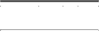
Multiple trim solutions may exist, mostly for the case of hover, especially when the blade airfoil sections are close to stall. In these situations, the rotor can provide the target thrust at multiple collective settings. This phenomenon is a result of the poststall airfoil lift characteristics, and a hypothetical example is illustrated in Fig. 2. The target lift coefficient is assumed to be 1.0, shown by the dashed horizontal line in the top plot in the figure. If the initial guess is such that the working angle of attack is 5 deg (point A), then the trim solver increases the root collective until the working angle of attack is 8 deg (point B) to achieve the required amount of lift. The corresponding drag coefficient is found using the table lookup at 8 deg (bottom plot). If, however, the angle of attack corresponding to the initial guess happens to be a poststall incidence angle (point C), the trim solver will further increase the collective until the lift decreases to the

required value (point D). From the bottom plot, it is clear that the profile drag at point D is two orders of magnitude larger than the corresponding value at point B.

Both trim solutions may be feasible (in the present study, they only need to be trimmable), although it is clear to a human analyst that point B is the preferred solution, and point D might be dubious. Not only can this lead the optimizer to discard some otherwise good designs because the profile drag appears to be excessively high, but serious numerical problems can occur. In fact, if there is a group of closely spaced designs for which trim converges to the correct prestall solution for some and the spurious poststall solution for others, the resulting RBF-based response surface may exhibit such extreme oscillations that the entire optimization may fail.

To restrict the analysis to prestall points (like point B), trim convergence is performed with multiple starting guesses for the collective pitch setting with dynamic inflow. These calculations are inexpensive and are easily automated. The trim variables corresponding to the smallest shaft power among these cases are then provided as an initial guess for the more computationally expensive trim iterations with the free vortex wake. This procedure is sufficient to remove the spurious poststall trim solutions.

F. Use of Graphical Processing Unit/Compute Unified Device Architecture in the Analysis

It is computationally expensive to use the free vortex wake methodology for multiple rotors, especially for the present multiobjective design optimization. At any time instant, each of the Nv vortex line segments interacts with all the other segments, and the computational cost increases as N2v. In the present study, each of the eight blades of the coaxial rotor trails a vortex of length equal to eight turns or 2880 deg, with a 10 deg wake age discretization. For these values, the total number of vortex–vortex interactions at a given time step is in excess of 5.3 million. These calculations are repeatedly performed during the time-marching wake simulations within multiple nested loops, leading to significant runtimes (15–20 min for trim convergence of one design at hover when parallelized over the individual cores of a quad-core central processing unit (CPU) using OpenMP (open multi-processing) directives) on a quad-core desktop.

Nominal code acceleration (25 times over single-core CPU) was achieved by transferring the computation of vortex–vortex interactions to an NVIDIA 560Ti GPU, using PGI's (The Portland Group, Inc.) Fortran Compiler (which includes CUDA Fortran extensions allowing the usage of parallelization on CUDA-enabled GPUs). Bottlenecks imposed by induced velocity computation and summation operations were alleviated, respectively, by using simple parallelization and multistage parallelized reduction trees.

Additional time savings were obtained in high-speed forward flight by exploiting knowledge of the flow physics. The 220 kt cruise condition corresponded to an advance ratio of μ 0.6, at which the

tip vortices were convected away from the rotors extremely quickly (compared to hover); and two turns of the tip vortex wake were sufficient to obtain an accurate representation of the inflow at the rotor disks, leading to a 16-times acceleration (compared to the case with eight turns) over and above the 25 times afforded by the GPU.

The GA optimization algorithm and RBF interpolation introduce additional overheads that are comparable to the runtimes for the objective function evaluations. On average, approximately 300 precise objective function evaluations (150 at hover and 150 at cruise), corresponding to the precise analysis of 150 designs, could be performed in a 24 h period when running unattended. All calculations are performed on a single off-the-shelf desktop computer with one graphics card.

V.Results

This section presents results for two multiobjective optimizations. The first is based on the six design variables listed in Table 1. The second is an eight-design-variable optimization obtained by adding hover rotor speed ΩH and rotor radius R. Selected characteristics of the aircraft are shown in Table 2.

A. Six-Design-Variable Optimization

1. Pareto Frontiers

The converged Pareto frontier is shown in Fig. 3. The hover anchor point corresponds to a hover power of FH 2215 HP and a cruise

FC 3024 HP. The design is always driven by the cruise power requirements. The figure also shows the line corresponding to equal hover and cruise powers, FC FH; and the entire frontier lies below the curve. It should be kept in mind that the configuration used in this study is not optimized for high-speed flight, and it has a relatively

Table 2 Selected aircraft characteristics

3200

Hover power

Hover power = Cruise power 3000

2800 Cruise

optimum

2600

2400

2200

Hover

Other (nonoptimal) designs optimum Pareto frontier

Cruise power (HP)

Fig. 3 Pareto frontier for the six-design-variable case.

high parasitic drag. A more suitable configuration will have lower equivalent flat-plate area, which will move the frontier to the left in the figure, and hover power requirements may dominate in some portion of the frontier.

There is a clear tradeoff between designs optimized for hover and for cruise. The frontier is very steep in the vicinity of the cruiseoptimum design, and the last 50–100 HP reduction in cruise power is paid with an increase in hover power by almost 400 HP. An equivalent trend is seen near the hover-optimum design: the last 50 HP of hover power reductions are obtained with a group of designs that may differ by about 400 HP of the cruise power required. Mathematically, not all of them are on the frontier, which can however be intuitively continued to slightly above 3800 HP of cruise power.

Extracting the Pareto frontier required 1112 precise objective function evaluations (high-fidelity performance analysis with free wake), of which 936 could be trimmed and 30 defined the frontier. Performing these objective function evaluations, as well as the optimization overhead, required one week of computational time on one desktop computer equipped with one GPU used for parallel calculations. It could be seen that the optimization procedure concentrated the designs in the region of the frontier. This implied the following:

1)A large number of intermediate designs were good designs, and relatively few were poor or untrimmable.

2)The accuracy of the RBF-based response surface was better in the region where it counted most, i.e., near the frontier.

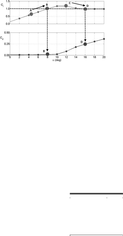
Figure 4 shows convergence information (namely, the frontiers every 200 designs) plus the final frontier for 1112 designs. These are precise frontiers, i.e., they are extracted from the all the precisely analyzed, trimmed designs available up to that point. Note that the frontier has essentially converged in the cruise-optimum region after

600designs, whereas 200–400 more are required for the hoveroptimum portion.

For subsequent analyses, it is interesting to also consider nearoptimal designs. Figure 5 shows the designs at distances of 25, 50, 100, and 200 HP from the Pareto frontier. A design is said to be at a distance (say, of 25 HP) if it is contained in the band obtained by translating the frontier by 25 HP: first along the y axis, and then along the x axis.

2.Design Trends

In Fig. 6, the hover power required and the blade twist are plotted as a function of cruise power required for all the designs on the Pareto frontier. Moving to the right and to the left on the horizontal axis (cruise power) means moving toward hoverand cruise-optimized designs, respectively. The figure indicates that lower (more positive)

Fig. 4 Convergence of the Pareto frontier for the six-design-variable case.

Cruise power (HP)

Fig. 5 Near-optimal designs for the six-design-variable case.

Cruise power (HP)

Fig. 6 Blade twist along the Pareto frontier.

Fig. 7 Blade twist along the Pareto frontier, including near-optimal designs.

twist is best for configurations that are more suitable for forward flight, whereas higher twist is better for hover. The curve fit approximates the designs very well.

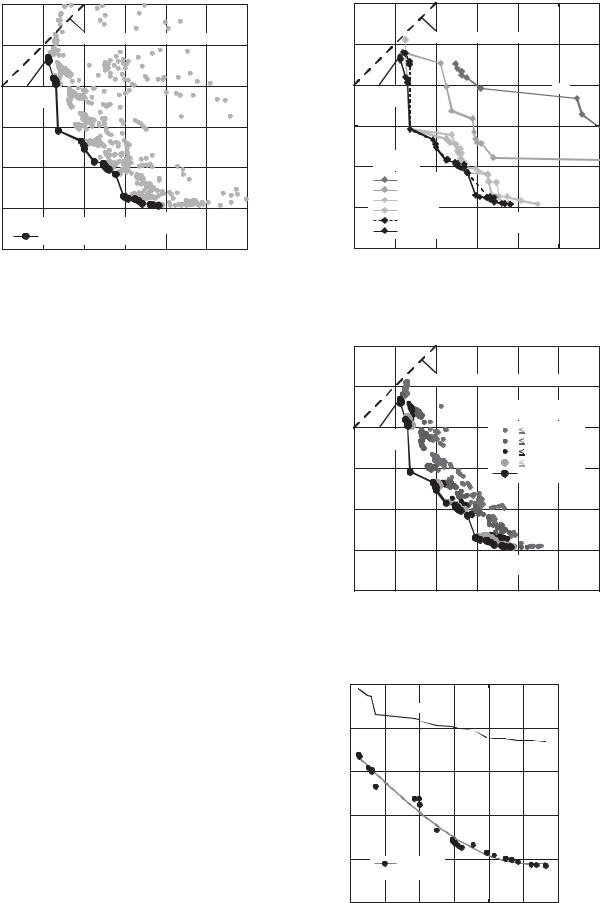
Figure 7 is similar to Fig. 6, except that the near-optimal designs have been added. The overall trends clearly remain the same. Optimal and near-optimal designs remain grouped in a relatively narrow band, about 2–3 deg wide, in traversing the Pareto frontier.

Figure 8 shows twist values after binning. The plot is obtained as follows. The range of values taken by the design variable (twist in this case) is scaled so that upper and lower bounds are set to one and zero, respectively. The range is divided into four intervals, or bins, of equal size, and the values corresponding to each design are symbol-coded. This results in a map of how a given design variable behaves throughout the objective function space. Taking a line parallel to the vertical (or hover power) axis and sliding toward the left shows the behavior of the design variable required for a reduction of cruise power. Taking a line parallel to the horizontal (or cruise power) axis and sliding it down shows the behavior required for a reduction of hover power.

With this in mind, Fig. 8 shows that twist progressively decreases (in absolute value) to achieve minimum cruise power, and it does so smoothly, transitioning through the various bins. The trend for minimum hover power is the opposite [i.e., a progressive increase

Cruise power (HP)

Fig. 9 Blade root chord along the Pareto frontier.

(in absolute value)] and with an equally smooth transition through the range of values. Overall, considering Figs. 6–8, blade twist can be considered as a numerically “well-behaved” variable, which changes smoothly while traversing the Pareto frontier and transitions equally smoothly through its range of values as each of the two objective functions is minimized.

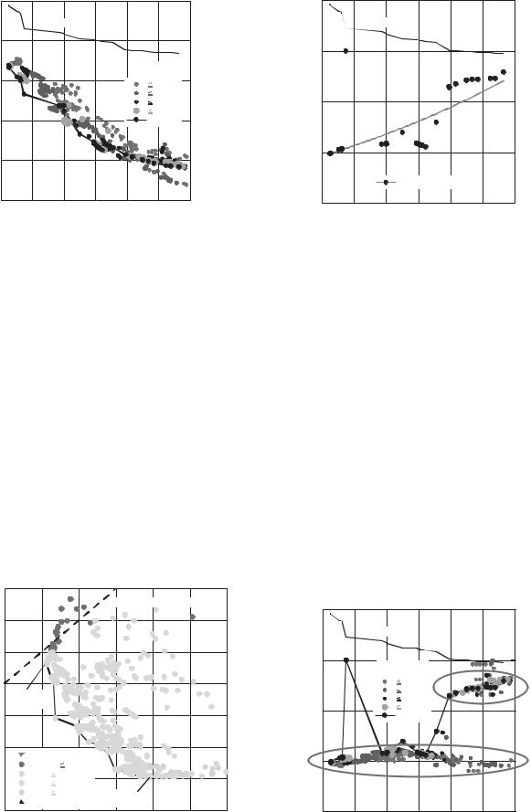
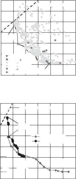
Figure 9 shows the behavior of the root chord along the Pareto frontier, and it is otherwise similar to Fig. 6. The general trend is for a wider chord blade for minimum hover power and a narrower chord blade for minimum cruise power. The low-order curve fit is a fair approximation to the designs along the frontier, but there is clearly more scatter than for twist in Fig. 6. Additionally, there is a design, at the upper bound of 4 ft, which clearly appears as an outlier.

A greater insight can be obtaining by adding the near-optimum designs to the plot, as is done in Fig. 10. The figure clearly shows that there are two distinct families of designs corresponding to two different engineering solutions: one with a wider chord of about 3.5 ft, and another with a narrower chord of about 2 ft. As the tradeoff is moved from cruise-optimum (left portion of the plot) to optimum hover (right portion of the plot), the narrow chord solution is preferable, but then it is better to switch to the wider chord. For low hover power, both engineering solutions are good, and a gradientbased optimizer will generally find one and not the other, depending on how it is started, and may very well give the wrong answer. A human designer might miss one of them too. The optimizer developed in the present study captures both, and it switches from one

3200

3000

2800

2600

Cruise power (HP)

Fig. 11 Blade root chord along the Pareto frontier, including nearoptimal designs.

to the other as needed. It also captures the outlier with a 4 ft chord, which lies on the Pareto frontier, and may belong to yet a third different family of designs.

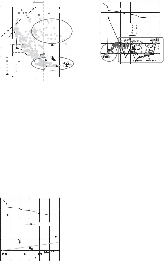
The situation is especially clear in the plot of the binned value of the root chord; see Fig. 11. By taking a line parallel to the y axis (dashed line in the figure) and sliding it to the left, it is possible to see how the chord should change to minimize cruise power. Initially, there seem to be two different strategies: one with the larger chord (encircled by lower oval), and another with the smaller chord (encircled by larger upper oval). Then it becomes obvious that the better strategy is to keep the root chord small. From an optimization point of view, if a gradient-based optimizer happened to start in the wide-chord region (for example, because the hover configuration was optimized first), it would probably be trapped in the local minimum (at about 3400 HP) and not be able to find the global minimum for cruise power (at about 3000 HP).

It is also interesting to consider the point on the Pareto frontier marked in Fig. 11 by the dashed rectangle. This is a design that appears as an outlier in Fig. 10. The root chord is at its upper bound. The optimizer manages to locate it even if all the designs in a broad region around it have much lower root chord values: between 25 and 50% of the respective ranges.

Figure 12 shows the wing root angle for the designs on the Pareto frontier and a corresponding trend line. There is a lot of scatter around

Cruise power (HP)

Fig. 12 Wing root angle along the Pareto frontier.

Fig. 13 Wing root angle along the Pareto frontier, including nearoptimal designs.

the trend line, which is simply drawn by hand to reflect the general behavior, and ignores a design “outlier,” corresponding to the same design that is an outlier for the blade root chord, at a wing root angle of about 13 deg.

When all the near-optimal designs are added, as shown in Fig. 13, a particular trend emerges. The root wing angle determines the wing lift and lift share between the rotor and wing. In the simplified simulation model used in this study, the wing does not generate lift in hover or download due to the aerodynamic interaction with the rotor; therefore, this variable does not affect hover power but only cruise power. It is interesting to follow the behavior of the optimal and nearoptimal designs, starting from the hover optimum and moving toward the left, toward the cruise optimum. Initially, there is a broad area (marked by the rectangle on the plot) where the angle stays in a band between about 4.5 and 9 deg but with a seemingly uniform random distribution. This is because there is no preferential value for hover because the wing root angle does not affect hover power. Getting closer to the cruise optimum (marked by an oval on the plot), the behavior becomes much more defined, and the spread is reduced. Also note the design on the Pareto frontier at about 13 deg. Therefore, the wing root angle is a design variable with a behavior that introduces two potential difficulties for gradient-based optimizers. First, because the design variable does not affect one objective function, all the corresponding derivatives (gradient, Hessian, etc.) are zero, and the Hessian is only positive semidefinite. Second, because there are at least two potential local minima, a gradient-based optimizer will be “trapped” in one or the other, and it will fail to identify both simultaneously.

The binned representation of root wing angle (Fig. 14) shows an essentially uniform distribution of symbols. This means that the design variable stays more or less in the same range throughout the design space.

B. Eight-Design-Variable Optimization

The same design optimization problem was solved with two extra variables added, namely, hover rotor speed ΩH and rotor radius R. The addition of the variables required an additional 534 precise objective function evaluations.

The Pareto frontiers for the sixand eight-design-variable cases are compared in Fig. 15. Hover power improves by almost 300 HP. Optimum cruise power, on the other hand, stays essentially constant. Some of the hover power reduction is due to the inclusion of hover rotor speed, which does not affect cruise power. The rest is due to the inclusion of rotor radius, which does affect cruise power. The combined effect is such that there is a substantial cruise performance penalty for the hover performance improvement, and such a design may prove unusable in practice. Note that the cruise power on the

Cruise power (HP)

Fig. 14 Wing root angle along the Pareto frontier, including nearoptimal designs.

Cruise power (HP)

Fig. 15 Pareto frontiers for the sixand eight-design-variable cases.

frontiers is about the same for the six-DVand eight-DV cases up to the six-DV anchor point.

Design optimizations with more than eight design variables are not attempted in this study. Response-surface-type methods tend to be subject to the “curse of dimensionality,” and it is possible that somewhere between 20 and 50 design variables can represent the practical maximum size of the problem. That number of design variables may not be sufficient to cover a realistic rotorcraft design problem, but it might be sufficient (possibly with a judicious use of design-variable linking techniques) to identify all the meaningful local optima of the design. The optimization could then be completed with gradient-based methods, which are far more efficient and capable of dealing with far larger numbers of design variables (although they can only guarantee convergence to a local optimum).

VI. Conclusions

The paper presented the results of a rotorcraft preliminary design problem for a coaxial configuration with lift and thrust compounding, solved as a multiobjective design optimization problem. An optimization methodology was developed that transformed the basic

problem into a sequence of approximate optimization problems, in which approximate Pareto frontiers were calculated based on response surfaces obtained from radial basis function interpolation of all the designs analyzed precisely, and was available at every step of the sequence. The approximate Pareto frontiers were computed using a genetic algorithm. The designs were analyzed using a highfidelity rotorcraft analysis that included nonlinear finite element models of the rotor blades and a free vortex wake model of the rotor inflow.

The results presented indicated the following:

1)The preliminary design optimization problem could be effectively solved using formal numerical design optimization techniques, which therefore could complement the classical methodology of multiple parameter sweeps, in a nested loop approach, until an optimal configuration was reached. The optimizer quantified the design tradeoffs in the form of Pareto frontiers, and it provided insight into the effects of the design parameters on the conflicting objective functions.

2)With appropriate implementation logic, the design optimization leading to the derivation of the Pareto frontiers could be carried out by the computer completely unattended: in particular, with no analyst intervention required to select the most appropriate combination of parameters.

3)The optimization methodology proved sufficiently robust to deal with potential numerical difficulties such as multiple local optima and insensitivity of one objective function to some design variables.

4)The optimization methodology proved computationally efficient enough to allow the use of high-fidelity analyses throughout the optimization rather than just for verification of selected designs. This was achieved on an off-the-shelf desktop computer. Use of GPU/CUDA computing contributed to the computational efficiency of the procedure.

The use of formal design optimization techniques promises to alleviate the designer’s burden of carrying out the multiple parameter sweeps required in conceptual and preliminary design. The designer’s role remains as important as ever in properly setting up the design optimization problem [selection of objective function(s), design variables, constraints], in ensuring a proper execution logic so that the optimization can proceed with as few interruptions as possible, in analyzing the final results, and in making the final configuration selections based on the tradeoffs quantified by the optimization.

Acknowledgments

This research work was conducted under the United States/Israel Rotorcraft Project Agreement. The authors would like to thank Jeffrey Sinsay of the U.S. Army Aeroflightdynamics Directorate, NASA Ames Research Center, for providing a formulation of the coaxial rotorcraft design problem, a simplified version of which was used in the paper. Extensive discussions with Omri Rand of the Technion–Israel Institute of Technology are gratefully acknowledged.

References

[1] Celi, R., “Recent Applications of Design Optimization to Rotorcraft—A Survey,” Journal of Aircraft, Vol. 36, No. 1, Jan.–Feb. 1999,

pp.176–189. doi:10.2514/2.2424

[2]Ganguli, R., “A Survey of Recent Developments in Rotorcraft Design Optimization,” Journal of Aircraft, Vol. 41, No. 3, May–June 2004,

pp.493–510.

doi:10.2514/1.58

[3]Orr, S. A., and Narducci, R. P., “Framework for Multidisciplinary Analysis, Design, and Optimization with High-Fidelity Analysis Tools,” NASA CR-2009-215563, Feb. 2009.

[4]Johnson, W., and Sinsay, J. D., “Rotorcraft Conceptual Design Environment,” 3rd International Basic Research Conference on Rotorcraft Technology, American Helicopter Soc. International, Inc., Alexandria, VA, Oct. 2009, https://ntrs.nasa.gov/search.jsp? R=20100026007.

[5]Sinsay, J. D., and Johnson, W., “Toward Right-Fidelity Rotorcraft Conceptual Design,” AIAA 48th Aerospace Sciences Meeting, AIAA Paper 2010-2756, Jan. 2010.

[6]Johnson, W., Yeo, H., and Acree, C. W., Jr., “Performance of Advanced Heavy-Lift, High-Speed Rotorcraft Configurations,” AHS International Forum on Rotorcraft Multidisciplinary Technology, American Helicopter Soc. International, Inc., Alexandria, VA, Oct. 2007.

[7]Yeo, H., and Johnson, W., “Aeromechanics Analysis of a Heavy Lift Slowed-Rotor Compound Helicopter,” Journal of Aircraft, Vol. 44, No. 2, March–April 2007, pp. 501–508.

doi:10.2514/1.23905

[8]Johnson, W., Moodie, A. M., and Yeo, H., “Design and Performance of Lift-Offset Rotorcraft for Short-Haul Missions,” American Helicopter Society Future Vertical Lift Aircraft Design Conference, American Helicopter Soc. International, Inc. Paper FVL-2012-010, Alexandria, VA, Jan. 2012.

[9]Moodie, A. M., and Yeo, H., “Design of a Cruise-Efficient Compound Helicopter,” Journal of the American Helicopter Society, Vol. 57, No. 3, 2012, Paper 032004.

doi:10.4050/JAHS.57.032004

[10]Rand, O., and Khromov, V., “Compound Helicopter: Insight and Optimization,” American Helicopter Society 69th Annual Forum, Phoenix, AZ, June 2013.

[11]Simpson, T. W., Toropov, V., Balabanov, V., and Viana, F. A. C., “Design and Analysis of Computer Experiments in Multidisciplinary Design Optimization: A Review of How Far We Have Come—Or Not,” 12th AIAA/ISSMO Multidisciplinary Analysis and Optimization Conference, AIAA Paper 2008-5802, Sept. 2008.

[12]Jones, D. R., “A Taxonomy of Global Optimization Methods Based on Response Surfaces,” Journal of Global Optimization, Vol. 21, No. 4, 2001, pp. 345–383.

doi:10.1023/A:1012771025575

[13]Gutmann, H. M., “A Radial Basis Function Method for Global Optimization,” Journal of Global Optimization, Vol. 19, No. 3, 2001, pp. 201–227.

doi:10.1023/A:1011255519438

[14]Tritschler, J., “Contributions to the Characterization and Mitigation of Rotorcraft Brownout,” Ph.D. Dissertation, Dept. of Aerospace Engineering, Univ. of Maryland, College Park, MD, 2012.

[15]Wilson, B., Cappelleri, D., Simpson, T. W., and Frecker, M., “Efficient Pareto Frontier Exploration Using Surrogate Approximations,”

Optimization and Engineering, Vol. 2, No. 1, 2001, pp. 31–50. doi:10.1023/A:1011818803494

[16]Howlett, J. J., “UH-60A Black Hawk Engineering Simulation Program: Volume I—Mathematical Model,” NASA CR 166309, Dec. 1981.

[17]Celi, R., “HeliUM 2 Flight Dynamic Simulation Model: Development, Technical Concepts, and Applications,” AHS 71st Annual Forum, American Helicopter Soc. International Inc. Paper 71-2015-368, Alexandria, VA, May 2015.

[18]Celi, R., “Helicopter Rotor Blade Aeroelasticity in Forward Flight with an Implicit Structural Formulation,” AIAA Journal, Vol. 30, No. 9, Sept. 1992, pp. 2274–2282.

doi:10.2514/3.11215

[19]Johnson, W., Helicopter Theory, Dover, New York, 1994, pp. 214– 216.

[20]Bagai, A., and Leishman, J. G., “Free-Wake Analysis of Tandem, TiltRotor and Coaxial Rotor Configurations,” Journal of American Helicopter Society, Vol. 41, No. 3, July 1996, pp. 196–207. doi:10.4050/JAHS.41.196

[21]Leishman, J. G., and Syal, M., “Figure of Merit Definition for Coaxial Rotors,” Journal of the American Helicopter Society, Vol. 53, No. 3, July 2008, pp. 290–300.

doi:10.4050/JAHS.53.290

[22]Leishman, J. G., and Ananthan, S., “An Optimum Coaxial Rotor System for Axial Flight,” Journal of the American Helicopter Society, Vol. 53, No. 4, Aug. 2008, pp. 366–381.

doi:10.4050/JAHS.53.366

[23]Leishman, J. G., “Aerodynamic Performance Considerations in the Design of a Coaxial Proprotor,” Journal of the American Helicopter Society, Vol. 54, No. 1, Jan. 2009, Paper 12005. doi:10.4050/JAHS.54.012005

[24]Syal, M., and Leishman, J. G., “Aerodynamic Optimization Study of a Coaxial Helicopter Rotor,” American Helicopter Society 65th Annual Forum, American Helicopter Soc. International, Inc. Paper 65-2009- 000097, Alexandria, VA, May 2009.

[25]McCormick, B. W., Aerodynamics, Aeronautics, and Flight Mechanics, Wiley, New York, 1979, p. 137.

[26]Tritschler, J., Syal, M., Celi, R., and Leishman, J. G., “A Methodology for Rotorcraft Brownout Mitigation Using Rotor Design Optimization,” AHS 66th Annual Forum, American Helicopter Soc. International, Inc. Paper 66-2010-000427, Alexandria, VA, May 2010.