International Short-Term Financing and Investment 251

(1 + e_y ⁾ > (1 + L ) 291

(1+f ) 300

(1+f ) 302

International Long-Term Financing, Capital Structure and the Cost of Capital 284

D = Z D, 283

E = Z 283

k = Z 289

International Long-Term Portfolio Investment 296

Rj,t = b 0,j + b 1, jR m,t + b 2,j$t + e j,t (11.40) 311

dL 319

dm ₁ -¹'—-¹'-²'"² --v-^"³ '-³ (1149) 319

+ 2ct(S 1, S ₄)w 4 +1 1 = 0 319

= 2w3 s ² (S3 ) + 2s(S 1 , S3 )w 1 + 2s(S2 , S3 )w2 320

+ 2s(S 3 , S₄ )w 4 +2 1 = 0 = 2w4 s ² (S4 ) + 2s(S 1 , S4 )w 1 + 2s(S 2 , S4 )w2 + 2s(S 3 , S4 )w 4 + 2 2 = 0 320

= w 1 + W2 + w 3 -1 = 0 320

w' = [w 1 w 2 w 3 w 4 2 1 2 2] and 331

Foreign Direct Investment 344

i 341

References 341

i 361

Index 363

Figure 1.3 shows the effect of two-currency arbitrage in the presence of fixed brokerage fees when the arbitrager buys y in B and sells it in A. Demand increases in B and supply increases in A, leading to a rise in the exchange rate in B and a fall in A. In this case, however, arbitrage does not come to an end when the exchange rates are equal in the two financial centres, but when the differ­ence between them is equal to the sum of brokerage fees incurred in both finan­cial centres, (b a + b b ). Figure 1.4 shows what happens to the no-arbitrage line when there are fixed brokerage fees. A band, 2( b a + b b ) wide, will be created around the original no-arbitrage line. The upper limit of the band is defined by equation (1.7), whereas the lower band is defined by equation (1.9). Points within the band but off the original no-arbitrage line indicate that while the exchange rates are not equal across financial centres, arbitrage is not profitable because arbitrage profit will be consumed by brokerage fees. Points falling outside the band define profitable arbitrage operations. Above the upper limit, arbitrage is profitable by buying y in B and selling it in A. Below the lower limit, arbitrage is profitable by buying y in A and selling it in B.

FIGURE 1.3 The effect of two-currency arbitrage in the presence of brokerage fees. Sa (x/y)

Assume now that brokerage fees depend on the size of the transactions, such that they are charged at the rates of b a and b b in financial centres A and B respectively. If Sa > Sb, then arbitragers will buy y in B and sell it in A. In this case the profit realised from arbitrage is

p = Sa (1 - b A ) - Sb(1 + b B )

(1.10)

(1.11)

which means that arbitrage will be profitable (p > 0) if

"1 + b B

^SA > ^SB

¹ - b A

Alternatively, if Sa < Sb, then arbitragers will buy y in A and sell it in B. In this case the profit realised from arbitrage is

(1.12)

(1.13)

p = Sb(1 - b B ) - Sa (1 + b A ) which means that arbitrage will be profitable if

" 1 - b b

^SA < ^SB

¹ + b A

Hence the no-arbitrage lines associated with (1.11) and (1.13) respectively are

(1.14)

"1 + b B

^SA = ^SB

¹ - b A

and

1 - b B

(1.15)

^SA = ^SB

¹ + b A

Figure 1.5 shows what happens to the no-arbitrage line in this case. Notice that since 0 < b_A < 1 and 0 < b _B < 1, it follows that (1 + b _B )/(1 - b_A ) > 1, while (1 - b b )/(1 + b a ) < 1. Diagrammatically, equations (1.14) and (1.15) are repre­sented in Figure 1.5 by two lines intersecting with the original no-arbitrage line at the origin, with one being steeper (1.14) and the other flatter (1.15). Points within the triangular area define unprofitable arbitrage, as any profit realised from the difference in the exchange rates across the financial centres will be consumed by brokerage fees. Any point above or below the triangular area indicates a profitable arbitrage opportunity.

Two-currency arbitrage in the presence of taxes

Here we consider two kinds of tax: capital gains tax and Tobin tax. We start with the former. Suppose that capital gains tax is imposed on the profits real­ised from two-currency arbitrage in the financial centre where the profit is realised. It is easy to show that the presence of capital gains tax has no effect on the no-arbitrage line, because the only effect of the tax is to reduce the profit received by the arbitrager. As long as there is a discrepancy between the exchange rates, arbitrage will be profitable, though less so than in the absence of the tax. Arbitrage will not come to an end unless the discrepancy between the exchange rates disappears.

Sa (x/ y)

FIGURE 1.5 The no-arbitrage zone in the presence of progressive brokerage fees.

Sb (x/y)

If the rate of capital gains tax is t, then the after-tax arbitrage profit obtained by buying y in B and selling it in A is

(1.16)

(1.17)

p = (1 -r)[S_A - S_B] in which case the no-arbitrage line is given by (1 - t)[SA- Sb ] = 0

which is equivalent to (1.4). Notice that dp/dt < 0.

Tobin tax was suggested by a Noble laureate, James Tobin, as a measure that would reduce the volatility in the foreign exchange market. It is imposed as a percentage of the value of the transaction, and hence it has the same effect as imposing brokerage fees on the buying and selling operations.

Two-currency arbitrage with capital controls

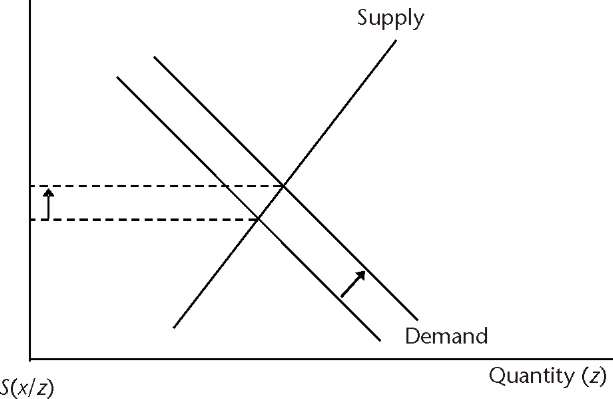
What happens if capital controls are imposed in one financial centre. If the transfer of capital is not allowed for financial transactions then arbitrage is not possible, and the divergence between the exchange rates in the two financial centres will persist. Nothing will happen to shift the supply and demand curves as in Figure 1.1. However, if capital controls are partial, the amount of capital allowed to be transferred from one financial centre to another may be inadequate to shift the supply and demand curves to the extent necessary to eliminate the discrepancy between the exchange rates. In this case, the

5 (x/y)

Supply

Demand

FIGURE 1.6 The effect of two-currency arbitrage in the presence of partial capital controls.

Supply

Quantity (y)

Quantity (y)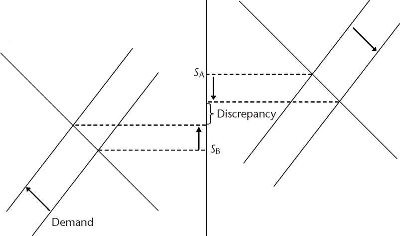

exchange rates in the two financial centres will approach each other, but they will not be equal. This situation is explained in Figure 1.6.

Two-currency arbitrage in the presence of the bid-offer spread

(1.18)

Let Sb,A and Sb,B be the bid rates, and S_a,A and S_a,B the offer rates in financial centres A and B respectively (still measured as S(x/y)). In the presence of the bid-offer spread, arbitragers buy (from market makers) at the higher offer rate and sell (to market makers) at the lower bid rate (note that Sb < S_a). Thus, the bid rate is determined by the demand of market makers and the supply of arbi­tragers. Conversely, the offer rate is determined by the demand of arbitragers and the supply of market makers. The bid and offer rates are related by the equation

Sa = Sb(1 + m)

where m is the bid-offer spread expressed as a percentage of the bid rate. For simplicity, we will assume that the bid-offer spread in financial centre A is equal to that prevailing in financial centre B.

(1.19)

Suppose now that the arbitrager wants to buy y in B and sell it in A. In this case arbitrage will be profitable if

^p = ^Sb,A ^{- S}a,B > ⁰ which means that the no-arbitrage condition is given by

Sb,A = Sa,B (1.20)

This situation is illustrated in Figure 1.7. Arbitragers buy y in B at S_a,B and sell it in A at Sb,A. The process leads to a shift in the arbitragers' demand curve in B, causing a rise in S_a,B and to a shift in the arbitragers' supply curve in A, causing a fall in Sb,A. The process continues until the two rates are equal. If only these changes take place, the bid-offer spread must rise in both A and B, and there is no reason why this should happen. In order that the spread stays at the same level, Sb,B must rise and S_a,A must fall. The following line of reasoning explains why this could take place. As Sa,B rises, market makers find it profitable to increase the supply of y. To do this, they must obtain larger quantities of y by

A: Demand of arbitragers and A: Demand of market makers and

B: Demand of arbitragers and B: Demand of market makers and

supply of market makers supply of arbitragers

FIGURE 1.7 The effect of two-currency arbitrage in the presence of bid-offer spread.

buying it from customers. Thus the market makers' demand curve shifts, leading to an increase in Sb,B. Similarly, as S^a declines, the market maker finds it cheaper to buy y, and the supply curve will shift to the left, leading to a fall in S_a,A.

Let us now consider the no-arbitrage condition in the presence of the bid-offer spread. Figure 1.8 shows a four-quadrant diagram, in which quad­rants 1 and 3 show the no-arbitrage condition, whereas quadrants 2 and 4 show the relationship between the bid and offer rates. Notice that the line representing the relationship between the bid and offer rates (passing through the second and fourth quadrants) is less steep than the 45° line because the bid rate is always lower than the offer rate. The first quadrant shows the no-arbitrage line represented by equation (1.20). Any point above

⁵bA

45° \	5b A = 5a, B
\ \
\ \ N
N \ \ \	5b A > 5a,B
\ \ \ \ v \ N. >	Buy y in B and sell it in A
\ \ \
\ N \ \ N
X. \ \ N \ \ \ N V \
5 ^ 5b a=!5: a
5a,A	5a,B s \ \ V \ —. \ 4. 5 = 5a,B 5b,B = 1 + a \ \ \ \ \ \ \ \ \ N \ \ \ \ \ N \ \ N \ N \ \ N
5b B > 5a, A	\ \ \
Buy y in A and sell it in B	X \ \ \ \ \ \ \
5bB = 5a,A	45°

FIGURE 1.8 The no-arbitrage condition in the presence of bid-offer spread.

the line implies profitable arbitrage, with profit given by equation (1.19). In the third quadrant, points below the no-arbitrage line represent profitable arbitrage opportunities taking the form of buying y in A and selling it in B. In this case the profit is

^p = ^Sb,B ^{- S}a,A ⁽¹.²¹⁾

The effect of the bid-offer spread is to reduce the profitability of arbitrage, since the spread is a transaction cost. Recall that equation (1.3) defines the arbi­trage profit as the difference between the exchange rate in A (the sell rate) and the exchange rate in B (the buy rate). These rates were not defined as bid or offer rates, so let us assume that they are the mid-rates, which means

^SA = i-[Sb,A + V ] a.22)

Sb = 2 [S_b,B + Sa,B] a.2³)

Arbitrage profit in the absence and presence of the bid-offer spread is given by equations (1.3) and (1.19) respectively. Since by definition

Sb,A < Sa (1.24) and

Sa,B > Sb (1.25) it follows that

^Sb,A ^{- S}a,B < ^SA ^{— S}B ⁽¹.²⁶⁾

which means that the presence of the bid-offer spread reduces the profit­ability of arbitrage, because the arbitrager has to buy at a higher rate and sell at a lower rate than otherwise.

Putting things together

Let us now consider the profitability of two-currency arbitrage in the presence of (i) bid-offer spread, (ii) fixed brokerage fees and (iii) Tobin tax. Consider the situation when the arbitrager buys y in B and sells it in A (equations 1.19 and 1.20). In the presence of fixed brokerage fees, b a and b b, and a Tobin tax, t, which is assumed to be equal in both financial centres, arbitrage profit is reduced to

^p = ^Sb,A ^{(1 -1) - b}A ^{- S}a,B⁽¹ + ^{t) - b} B (_{1 27})

= [Sb,A- Sa,B ](1 -1) -( b A+ b b)

which means that profit is reduced further (that is, on top of the reduction resulting from the bid-offer spread). Equation (1.27) implies a no-arbitrage condition that is expressed as

^Sb,A ^{- S}a,B = —A I— ⁽¹.²⁸⁾

which means that, for profitable two-currency arbitrage, the gap between the bid rate in A and the offer rate in B must be greater than ( b a + b b )/(1 -1)

1.3 THREE-CURRENCY ARBITRAGE

Three-currency arbitrage, also known as triangular arbitrage and three-point arbitrage, works as follows. Given three currencies (x, y and z), three possible exchange rates exist: S(x/y), S(x/z) and S(y/z). Since we are in this case dealing with three exchange rates, we will resort to the original exchange rate nota­tion, which shows the units of measurement, as above. We say that the three exchange rates are consistent if

S(x / y) = (1.29)

S(y / z) ^{V f}

Now, let us see what happens if an arbitrager tries to make profit by moving from one currency to another, ending up with the first currency. If the arbi­trager ends up with one unit of the currency he or she started with, then arbi­trage profit will be made. In general, if the condition (1.29) is violated then arbitrage profit can be made by moving in a particular direction and a loss will be made by moving in the opposite direction.

So, let us start with one unit of currency x, conducting arbitrage in the following manner:

1. Selling x and buying y to obtain 1/[S(x/y)] units of y.

2. Selling y and buying z to obtain 1/[S(x/y)S(y/z)] units of z.

3. Selling z and buying x to obtain S(x/z)/[S(x/y)S(y/z)] units of x.

The profit realised from this operation (measured in units of x) is given by p = ^S(x/z) -1 (1.30)

^{S( x/}y^)S( y^/z)

If the condition represented by (1.29) is valid, it follows that p = 0, which means that (1.29) is the no-arbitrage condition. However, if

S( x/y) < (1.31)

^S( y^/z)

it follows that

b A_+b I 1 -1

S(x/z) > S(x/y)S(y/z) (1.32)

which means that p > 0. Hence, if the no-arbitrage condition (1.29) is violated, such that (1.31) is valid, then three-currency arbitrage will be profitable by the following sequence: x ® y ® z ® x.

Now, let us see what happens if the arbitrager follows the sequence x ® y ® z ® x, starting with one unit of x. This operation consists of the following steps

1. Selling x and buying z to obtain 1/[S(x/z)] units of z.

2. Selling z and buying y to obtain S(y/z)/[S(x/z)] units of y.

3. Selling y and buying x to obtain S(y/z)S(x/y)/[S(x/z)] units of x.

The profit realised from this operation is given by

p = ^{S( y/z)S( x/y)} -1 (1.33)

S(x/z)

Again, it is obvious that if (1.29) is valid then p = 0. In this case, profitable arbi­trage is indicated by the violation of (1.29) such that

S( x/y) > (1.34)

^S( y^/z)

because (1.34) implies that

S(y/z)S(x/y) > S(x/z) (1.35)

which means that p > 0.

Just like two-currency arbitrage, three-currency arbitrage leads to a restora­tion of the no-arbitrage condition via changes in the supply of and demand for the three currencies. Let us trace what happens in the first case, as represented by (1.31). With the aid of Figure 1.9, we can see that each of the three steps results in changes in the forces of supply and demand as follows:

1. An increase in the demand for y (the supply of x), so S(x/y) rises.

2. An increase in the demand for z (the supply of y), so S(y/z) rises.

3. An increase in the demand for x (the supply of z), so S(x/z) falls.

These changes in supply and demand will restore the equilibrium condition.

Three-currency arbitrage in the presence of bid-offer spreads

Let us see what happens if an arbitrager wants to follow the sequence x ® z ® y ® x in the presence of bid-offer spreads. The operation consists of the following steps:

1. Buying z against x at S_a(x/z) to obtain 1/[S_a(x/z)] units of z.

2. Buying y against z at Sb(y/z) to obtain Sb(y/z)/[S_a(x/z)] units of y.

3. Buying x against y at S_a(x/y) to obtain Sb(y/z)S_a(x/y)/[S_a(x/z)] units of x.

For this operation to be profitable, the following condition must be satisfied:

S(x/y)

FIGURE 1.9 The effect of three-currency arbitrage.

^Sb⁽y^/z)Sa ^(x/y⁾ > ₁

^Sa^{( x/z)}

which gives

p = %^(y/z)Sa^(x/y) - 1 (1.37)

Sa( x/z)

in which case, the no-arbitrage condition is

Sa(x/y) = S^ (1.38)

^Sb⁽ y^/z)

Likewise, it can be shown that the sequence x ® y ® z ® x can be profitable

if

^Sb(x/z) >1 (1.39)

^Sb^{( x/}y^)Sa⁽ y^/z)

which gives

p = ^{Sb( x/z)} -1 (1.40)

^Sb^{( x/}y^)Sa⁽ y^/z)

in which case, the no-arbitrage condition is

Sb( x/y) = SS^ (1.41) ^Sa⁽ y^/z)

Equations (1.38) and (1.41) are used to calculate the bid and offer cross exchange rates when currency z is the numeraire.

1.4 MULTI-CURRENCY ARBITRAGE

Consider arbitrage involving four currencies: x\, x^, x3 and x4 by following the sequence x 1 ® x2 ® x3 ® x4 ® x ₁ . Arbitrage consists of the following steps:

1. Buying x2 and selling x1 at S(xx/x2) to obtain 1/[S(xx/x2)j units of x2.

2. Buying x3 and selling x2 at S(x2/x3) to obtain 1/[S(x1/x2)S(x2/x3)] units of x3.

3. Buying x4 and selling x3 at S(x3/x4) to obtain 1/[S(x1/x2)S(x2/x3)S(x3/x4)] units of x4.

4. Buying x\ at S(x^/x4) to obtain S(x1/x4)/[S(x1/x2)S(x2/x3)S(x3/x4)] units of x\. This operation will be profitable if

p = ^{S( x} l^{/x 4)} -1 > 0 (1.42)

S(x 1/x2 )S(x2 /x3 )S(x3/x4 )

in which case the no-arbitrage condition is

S(x! /x4 ) = S(x 1/x2 )S(x2 /x3 )S(x3/x 4 ) (1.43)

S(Xi/x2 )S(X2 /x3 )S(X3/x4 )S(X Jx 1) = 1 (1-44)

In general, an n-currency arbitrage is profitable if the following no-arbitrage condition is violated:

S(x1/x2)S(x2/x3)S(x3/x4)...S(x„-1/x„)S(x„/x1) = 1 (1-45)

which means that even two-currency arbitrage can be represented as a special case of (1-45). If n = 2, the no-arbitrage condition reduces to

S(x1/x2)S(x2/x1) = 1 (1-46)

Chacholiades (1971) has shown that if three-currency arbitrage is not profit­able, then n-currency arbitrage is not profitable either. This means that for equa­tion (1-45) to be satisfied, a necessary and sufficient condition is

S(x1/x2)S(x2/x3)S(x3/x1) = 1 (1-47)

The proof of this proposition is based on mathematical induction- If (n-1)- currency arbitrage is not profitable, then n-currency arbitrage is not profitable either- For unprofitable n-currency arbitrage, equation (1-45) must hold- Since (n-1)-currency arbitrage is not profitable by assumption, the following equa­tion must be satisfied

S(x1/x2)S(x2/x3)S(x3/x4)---S(xn-2/xn-1)S(xn-1/x1) = 1 (1-48)

Dividing (1-44) by (1-48) we obtain

^S(xn-1 ^/xn ^)S(xn^/x 1⁾

= 1 (1.49)

S(x_n_ i /X i)

which, for n = 3, is equivalent to (1.47) because S(xx/x2) = 1/[S(x2/xx)]. Hence, if (1.47) and (1.48) are satisfied, (1.45) must also be satisfied, which proves the proposition.

Multi-currency arbitrage with bid-offer spreads

In the presence of bid-offer spreads, the operation takes the following form:

1. Buying x2 and selling x\ at S_a(xx/x2) to obtain 1/[S_a(xx/x2)] units of x2.

2. Buying x3 and selling x2 at S_a(x2/x3) to obtain 1/[S_a(x1/x2)S_a(x2/x3)] units of ^x3.

3. Buying x4 at S_a(x3/x4) to obtain 1/[S_a(x1/x2)S_a(x2/x3)S_a(x3/x4)] units of x4.

4. Buying x1 at Sb(x1/x4) to obtain Sb(x1/x4)/[S_a(x1/x2)S_a(x2/x3)S_a(x3/x4)] units of ^x1.

This operation will be profitable if

p = ^{Sb( x 1x 4)} -1 > 0 (1.50)

^Sa^(x 1 ^/x2 ^)Sa^(x2 ^/x3 ^)Sa^(x3^/x4 ⁾

in which case the no-arbitrage condition is

Sb(xx/x4) = Sa(xx/x2)Sa(x2/x3)Sa(x3/x4) (1.51)

or

Sa(x1/x2)Sa(x2/x3)Sa(x3/x4)Sa(x4/x1) = 1 (1.52)

because Sb(xx/x4) = 1/[S_a(x^xx)]. If the bid-offer spread is the same for all exchange rates, the condition becomes

Sb(xx/x2)Sb(x2/x3)Sb(x3/x4)Sb(xx/x4)(1 + m)⁴ = 1 (1.53)

Hence the n-currency no-arbitrage condition in the presence of bid-offer spread is given by

Sa(x1/x2)Sa(x2/x3)Sa(x3/x4)...Sa(x_n/x1) = 1 (1.54)

or

Sb(x1/x2)Sb(x2/x3)Sb(x3/x4)...Sb(x„/x1)(1 + m)ⁿ = 1 (1.55)

1.5 EXAMPLES

Table 1.1 reports some bilateral exchange rates as on 16 December 2001. We can use these figures to check whether or not the no-arbitrage conditions asso­ciated with three-currency, four-currency and five-currency arbitrage are valid.

Table 1.2 lists possible sequences for three-currency, four-currency and five- currency arbitrage, the associated conditions and whether or not the condi­tions are satisfied. The numbers appearing in the third column are the prod­ucts of the exchange rates as implied by the general no-arbitrage condition (1.45). The no-arbitrage condition will be satisfied if the product is 1, indi­cating zero profit. This is because unity signifies that the no-arbitrage condi­tion implies that when the arbitrager starts with one unit of a particular

TABLE 1.1 Exchange rates on 16 December 2001.

x/y	USD	SEK	DKK	NZD	EUR AUD
USD	1
SEK	10.54	1
DKK	8.2449	0.7819	1
NZD	2.3941	0.2271	0.2904	1
EUR	1.1073	0.1050	0.1343	0.4625	1
AUD	1.9296	0.1830	0.2340	0.8060	1.7246 1

Source: Bloomberg.

TABLE 1.2 Exampl	es of n-currency arbitrage.
Arbitrage	Sequence	Condition
Three-currency	SEK ® USD ® NZD ® SEK	0.9998
Three-currency	AUD ® EUR ® DKK ® AUD	0.9898
Four-currency	USD ® NZD ® DKK ® SEK ® USD	0.9997
Four-currency	EUR ® NZD ® SEK ® AUD ® EUR	0.9898
Five-currency	SEK ® USD ® DKK ® NZD ® EUR ® SEK	0.9994
Five-currency	AUD ® EUR ® NZD ® SKK ® DKK ® AUD	0.9900

currency, she ends up with one unit of the same currency. The calculation of the figures in the third column can be illustrated by reference to the first arbi­trage operation. In this case we have

1

S(SEK/USD)x S(USD/NZD)x S(NZD/SEK) = 10.5400 x —— x 0.2271

2.3941

= 0.9998

We can see that all of the numbers are close to one, implying the absence of profitable arbitrage operations if we assume that the slight difference between unity and the figures shown in the table is due to rounding. If it is not due to rounding, then there is still no possibility for profitable arbitrage because the difference is so small that it is bound to be consumed by transaction costs.

Let us now assume that there is a 0.1% bid-offer spread in all exchange rates, such that we have the following information:

S(SEK/USD) = 10.5295 -10.5505

S(NZD/USD) = 2.3917 - 2.3965

S(NZD/SEK) = 0.2269 - 0.2273

In this case, the no-arbitrage condition is checked as follows

1

S_a (SEK/USD)x S_a(USD/NZD)x S_a(NZD/SEK) = 10.5505 x —-—x 0.2273

2.3965

= 10008

which is again close to unity, implying the absence of profitable arbitrage.

I

i

CHAPTER 2

Covered and Uncovered Interest

Arbitrage

2.1 COVERED INTEREST ARBITRAGE WITHOUT DISTORTIONS

Covered interest arbitrage is an operation that is conducted in four markets involving two currencies: (i) the spot foreign exchange market, (ii) the forward foreign exchange market, (iii) the money market in currency x, and (iv) the money market in currency y. The objective is to make profit by going short on one currency and long on the other, while covering the long position in the forward market. When it matures, the long position is unwound and the proceeds are converted into the other currency at the forward rate agreed upon in advance. The proceeds are then used to meet the obligations arising from the short posi­tion, and any left over would then represent net arbitrage profit. Notice that the operation is risk-free in the sense that the decision variables are known at the time when the transaction is initiated.

Let S and F be the spot and forward exchange rates between currencies x and y measured as S(x/y) and F(x/y). Also let i_x and iy be the interest rates on x and y respectively, such that the maturities of the assets and liabilities under­lying i_x and iy (for example, deposits and loans) are identical to the maturity of the forward contract. We will assume a two-period model where t is the present time at which the operation is initiated and t+1 is the future when the long position, short position and the forward contract mature. Whether the arbitrager goes short on x and long on y or the other way round depends on the configuration of interest and exchange rates. A covered arbitrage opera­tion by going short on x and long on y (x ® y) consists of the following steps:

1. At time t, the arbitrager borrows one unit of x at i_x for a period extending between t and t + 1, when the forward contract matures.

2. The amount borrowed is converted at S, obtaining 1/S units of y. This amount is then invested at iy.

3. At t + 1, the value of the investment is (1/S)(1 + iy) units of y.

4. The x currency value of the investment converted at the forward rate is (F/ S)(1 + iy).

5. At t + 1 the loan matures, and the amount (1 + i_x) has to be repaid.

The net profit arising from this operation, which is also called the covered margin, is given by

^p = s ⁽¹+^{y^)-(1+ⁱx ⁾

Hence the no-arbitrage condition is

F

(2.1)

(2.2)

S ⁽¹ + ^ly ⁾ = ⁽¹ + ^lx )

The equality of the gross return on y and the cost of borrowing x (principal plus interest) after covering the foreign exchange risk by selling y forward, as represented by (2.2), is called covered interest parity (CIP). This relationship is an application of the law of one price to financial markets (identical financial assets should produce identical returns after covering the foreign exchange risk).

^ No-arbitrage line

Figure 2.1 shows the no-arbitrage condition represented by equation (2.2). The no-arbitrage line is represented by a 45° line passing through the origin. Any point above the line represents profitable arbitrage by going short on x and long on y (x ® y), whereas points below the line represent profitable arbi­trage by going short on y and long on x (y ® x).

S (1+ i y )

S (1+ iy) = (i + ix)

Profitable arbitrage

x ^ y

Profitable arbitrage

y ^ x

(1+ ix)

FIGURE 2.1 The no-arbitrage condition implied by CIP.

Suppose now that the interest rate and exchange rate configuration is such that the no-arbitrage condition is violated, as represented by a point above the no-arbitrage line. In this case, arbitrage will lead to changes in the forces of supply and demand as illustrated in Figure 2.2. The following will happen:

1. Demand declines in the money market for x-denominated assets, leading to a rise in i_x.

2. Demand rises in the money market for y-denominated assets, leading to a decline in iy.

3. The demand for currency y increases in the spot market, leading to a rise in the spot exchange rate, S.

4. The supply of currency y rises in the forward market, leading to a decline in the forward exchange rate, F.

These changes combined lead to a decline in the covered return on y and an increase in the cost of borrowing x. When they are equal, the covered margin is

x

	Demand
	Ay
t
	Supply

y

Demand

Supply

Money market (x)

	Supply
t \
	Demand

S(x/y)

F(x/y)

Money market (y)

	Supply
	/V
	Demand

Spot market Forward market

FIGURE 2.2 The effect of covered arbitrage.

equal to zero, and the no-arbitrage condition is re-established. Arbitrage comes to an end, as the new configuration of interest and exchange rates is represented by a point falling on the no-arbitrage line.

Other forms of the no-arbitrage condition

The no-arbitrage condition can be expressed differently by manipulating equation (2.2). First of all we could rewrite this equation in terms of the net amounts, by subtracting 1 from both sides of the equation, to obtain

F

S (1 + iy ) -1 = ix (2.3)

Another specification of the no-arbitrage condition can be obtained by deriving the value of the forward rate consistent with CIP, the so-called equi­librium or interest parity forward rate, from equation (2.2). In order to distin­guish between the actual forward rate (which prevails whether or not CIP holds) and the equilibrium rate, the latter is denoted F. Thus the CIP no-arbi­trage condition may be written as

F = F (2.4)

where

F = S

1 + i_x

^lx

(2.5)

¹ + ⁱy

which means that the interest parity forward rate, as represented by equation (2.5), is calculated by adjusting the spot rate for a factor reflecting the interest rate differential. Since

F

palgrave 1

palgrave 2

i 19

i 23

CHAPTER 3 44

Other Kinds of Arbitrage and Some Extensions 46

3.1 COMMODITY ARBITRAGE 46

^Py ,t+ 1^/Py ,t 55

3.2 ARBITRAGE UNDER THE GOLD STANDARD 61

3.3 ARBITRAGE BETWEEN EUROCURRENCY AND DOMESTIC INTEREST RATES 63

3.4 EUROCURRENCY-EUROBOND ARBITRAGE 74

3.5 ARBITRAGE BETWEEN CURRENCY FUTURES AND FORWARD CONTRACTS 52

3.6 REAL INTEREST ARBITRAGE 54

3.7 UNCOVERED ARBITRAGE WHEN THE CROSS RATES ARE STABLE 55

3.8 UNCOVERED INTEREST ARBITRAGE WHEN THE BASE CURRENCY IS PEGGED TO A BASKET 57

^ ^ 1=1 »j ^ j=1 and 57

E1= S ₀ - S j (3.40) 57

3.9 MISCONCEPTIONS ABOUT ARBITRAGE 83

CHAPTER 4 65

Hedging Exposure to Foreign Exchange Risk: The Basic Concepts 65

4.1 DEFINITION AND MEASUREMENT OF FOREIGN EXCHANGE RISK 65

4.2 VALUE AT RISK 69

4.3 DEFINITION AND MEASUREMENT OF EXPOSURE TO FOREIGN EXCHANGE RISK 74

4.4 TRANSACTION EXPOSURE 82

4.5 ECONOMIC AND OPERATING EXPOSURE 84

4.6 A FORMAL TREATMENT OF OPERATING EXPOSURE 95

dQ_py_ dPy Q 102

4.7 TRANSLATION EXPOSURE 123

Financial and Operational Hedging of Exposure to Foreign Exchange Risk 105

^Fb,t - ^Sb,t 123

^{p - K(F}a,t ^{- S}b,t+ 1 ⁾ 133

Measuring the Hedge Ratio 158

, ^s(DPu,t, ^DPA,t I^f t-1) ,_{t t} . 164

^h = ^ ^ r" = ^P(X 1,t , ^X 2 ,t ⁾ 164

^{s 2(D}P A,t^|f t-1 ⁾ 164

^DP u,t = t-1 + Z ^ai ^DP U,t-i +Z ^bi ^dPa ,t-i +^x 1,t ⁽⁶.³³⁾ 186

^DP A,t =^-bft-1 + Z ^ci ^DP U,t-i +Z ^d i ^DP A,t - i +^X 2 ,t ⁽⁶.³⁴⁾ 186

^s(DPU,t^{, D}PA,t I^f t-1^{, D}PU,t-i^{, D}PA,t-i⁾ 186

^s2 (^APA,t I^f t-1' ^APU,t-i ' ^APA,t-i ⁾ _{(6 35}) 186

I,t ' X 2,t ) / s(X i,t ) ^ 186

= P^(X 1't ' ^X 2 ,t ⁾ 186

_ P^(X 1,t ^{, X} 2 ,t^)s(X 1,t^)s(X 2 ,t^{) -2 (f} t-1^{1 A}P U,t-i^{, A}PA,t-i⁾ 187

^s2 (^X2 ,t ) + ^{b2 s 2} (f t-1^{1 A}PU,t-i^{, A}PA,t-i ) 187

Speculation in the Spot and Currency Derivative Markets 184

^Sb,t 198

^Sb,t ¹ + ^m 198

^Sb,t ¹ + ^E(mt+1⁾ 199

^{E( S}b,t+1 ⁾, S 200

if the position in x is available. If the funds have to be borrowed, the condition changes to 201

Speculation: Generating Buy and 209

Sell Signals 209

St = f (Xt) 257

where the vector of variables varies according to the underlying fundamental model. The current level of the exchange rate may deviate from the equilib­rium level because of the effect of random shocks that tend to have a tempo­rary effect. Hence the current level of the exchange rate may be represented by 258