

Laboratory work №2 Solution of Nonlinear Equations by the Bisection method and Chord method
2.1 Purpose of the work
This laboratory work helps students a) study of numerical methods for solving nonlinear equations; b) the use of MATLAB for solving nonlinear equations.
2.2 Tasks for laboratory work
To study the iterative methods(Bisection and Chord) for solving nonlinear equations
Make a program function to find the root of the Bisection and Chord methods.
Debug the program.
To carry out the individual task.
Save results of the work (the programs, listing of calculation) at your personal file.
Draw up report.
2.3 The basic theoretical knowledge
Equations that can be cast in the form of a polynomial are referred to as algebraic equations. Equations involving more complicated terms, such as trigonometric, hyperbolic, exponential, or logarithmic functions are referred to as transcendental equations. The methods presented in this section are numerical methods that can be applied to the solution of such equations, to which we will refer, in general, as nonlinear equations. In general, we will search for one, or more, solutions to the equation,
f(x) = 0.
You will study the Bisection and Chord algorithm in this laboratory work. In these methods we need to provide two initial values of x to get the algorithm started.
Because the solution is not exact, the algorithms for any of the methods presented herein will not provide the exact solution to the equation f(x) = 0, instead, we will stop the algorithm when the equation is satisfied within an allowed tolerance or error, ε. In mathematical terms this is expressed as
|f(xR)| < ε.
The value of x for which the non-linear equation f(x)=0 is satisfied, i.e., x = xR, will be the solution, or root, to the equation within an error of ε units.
2.3.1 Bisection method
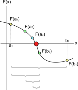
Figure 2.1 – Bisection method
On the picture 2.1 figure a few steps of the bisection method applied over the starting range [a1;b1]. The bigger dot is the root of the function.
The bisection method is a root-finding algorithm which works by repeatedly dividing an interval in half and then selecting the subinterval in which the root exists.
Suppose we want to solve the equation f(x) = 0. Given two points a and b such that f(a) and f(b) have opposite signs, we know by the intermediate value theorem that f must have at least one root in the interval [a, b] as long as f is continuous. The bisection method divides the interval in two by computing c = (a+b) / 2. There are now two possibilities: either f(a) and f(c) have opposite signs, or f(c) and f(b) have opposite signs. The bisection algorithm is then applied to the sub-interval where the sign change occurs, meaning that the bisection algorithm is inherently recursive.
Program of Bisection method is shown in listing 2.1.
Listing 2.1. File Bisection.m
function [x,k]=Bisection(f,a,b,eps)
%Data Input f – name m-file containing a description of the functions
% included in the nonlinear equation;
% a and b - left and right border of the segment localization
% of the root;
% eps – accuracy;
%Data Output x – root;
% k – number of iterations.
ya= feval(f,a); yb= feval(f,b);
if ya*yb>0
error('There are no roots on given interval');
end;
k=0;
while abs(a-b)>eps
k=k+1; x=(a+b)/2; fx=feval(f,x);
if fx==0
break;
elseif fa*fx<0
b=x; fb=fx;
else
a=x; fa=fx;
end;
end;
Example 2.1. Find the root of the equation
x4 - 11x3 + x2 +x +0.1 = 0
using the method of bisection.
1. Create a file Func.m(listing 2.2), containing a description of the function
f(x)= x4 - 11x3 + x2 +x +0.1
listing 2.2. File Func.m
function z=Func(x)
z=x.^4-11*x.^3+x.^2+x+0.1;
2. To separate the roots graph of the function by executing the following sequence of operators:
>>x1=-5;x2=15;
>>fplot(@Func,[x1 x2]); grid on

Figure 2.2 - Graph of the function f(x)= x4 - 11x3 + x2 +x +0.1 on interval [-5,15]
3. Refine the behavior of functions on the interval from -1 to 1(picture 2.3):
>>x1=-1;x2=1;
>>fplot(@Func,[x1 x2]); grid on
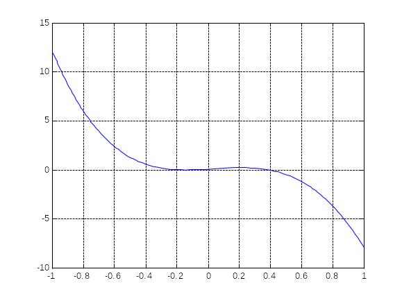
Figure 2.3 - Graph of the function f(x)= x4 - 11x3 + x2 +x +0.1 on interval [-1, 1]
4. Select one of the intervals localization – [-0, 1] and calculate the value of the root of the equation on this interval with accuracy ε=10^-5 by Bisection method:
>> eps=1.e-5;
>> [root,count_iter]=Bisection(‘Func’,0,1,eps)
root =
0.3942
count_iter =
17
5. Check the resulting value of the root:
>>y=Func(root)
y=
7.4926e-006
Example 2.2. The "manual" solution of nonlinear equation. Calculate the accuracy of the decision reached by the nonlinear equation
x sin(x) - 1 = 0
for 4 iterations.
We know that our zero lies between 0 and 2. Starting with a0=0 and b0=2 we compute
f(0) = -1,000000 and f(2) = 2*sin(2) – 1 = 0,818595.
Midpoint - x0 = (a0 +b0)/2 = 1 and f(1)=1*sin(1)-1= -0,158529. Consequently, the function changes sign on the interval [x0;b0] = [1;2].
Continue to perform compression of the left and assign a1 = x0, b1 = b0. Midpoint x1 = 1,5 and f(x1) = 0,496242. From f (1) = -0.158529 and f(1,5) = 0,496242 implies, that the root lies on the interval [a1; x1] = [1,0; 1,5]. The next step is compression of the right and assign a2 = a1 and b2 = x1. Thus we obtain a sequence {xk }, which converges to the root. Example calculations shown in Table 1.1.
Table 2.1 - The solution of the equation x sin(x) - 1 = 0 method of bisection
k |
The extreme left point, ak |
Midpoint, xk |
The extreme right point, bk |
The value of the function |
Accuracy at k iteration |
0 |
0 |
1 |
2 |
-0,158529 |
|
1 |
1,0 |
1,5 |
2,0 |
0,496242 |
2 |
2 |
1,0 |
1,25 |
1,50 |
0,185231 |
0,5 |
3 |
1,0 |
1,125 |
1,250 |
0,015051 |
0,25 |
4 |
1,0000 |
1,0625 |
1,1250 |
-0,071827 |
0,125 |