
- •Чисельні методи Використання MatLab
- •Затверджено
- •Contents
- •The purpose and the contents of laboratory works
- •Laboratory work №1 Programming in the environment of Matlab
- •1.1 Purpose of the work
- •1.2 The tasks to laboratory work
- •The basic theoretical knowledge
- •Global Variables
- •Passing String Arguments to Functions
- •Constructing String Arguments in Code
- •The eval Function
- •Vectorization
- •Preallocation
- •Anonymous Functions
- •Switch and case
- •Continue
- •The individual task to laboratory work
- •1.5 The task for self-examination
- •1. For opening the editor of the programs in MatLab it is possible to execute:
- •Laboratory work №2 Solution of Nonlinear Equations by the Bisection method and Chord method
- •2.1 Purpose of the work
- •2.2 Tasks for laboratory work
- •2.3 The basic theoretical knowledge
- •2.3.1 Bisection method
- •Figure 2.1 – Bisection method
- •Chord method
- •Figure 2.4 – Chord method
- •2.3.3 Matlab function fzero and roots
- •2.4 Individual tasks
- •2.5 Control questions
- •Laboratory work №3 Solution of Nonlinear Equations by the newton method and simple iteratIvE method
- •Figure 2.1 – Newton method
- •Figire 2.2 - Dependence of the number of iterations on the accuracy of methods for the bisection (upper line) and the Newton method (bottom line)
- •2.3.2 The method of simple iteration
- •A sufficient condition for the convergence of the iterative process
- •Individual tasks
- •Laboratory work №3 Solution system of Linear Algebraic Equations
- •3.3.1 Direct methods
- •Inverse matrix:
- •3.3.2 Iterative methods
- •Condition number of a
- •3.4 Individual tasks
- •3.5 Control questions
- •Solving systems of nonlinear equations
- •5.1 Purpose of the work
- •5.2 Tasks for laboratory work
- •5.3 The basic theoretical knowledge
- •5.3.1 Newton method to solve systems of non-linear equations
- •5.3.2 Matlab function for Newton method for a system of nonlinear equations
- •5.3.3 The matlab routine function fsolve
- •Input Arguments
- •Individual tasks
- •5.5 Control questions
- •List of the literature
- •Appendix a.
- •Individual tasks to Lab number 1, 2
- •Appendex b. The task for self-examination to Lab number 1, 2
Inverse matrix:
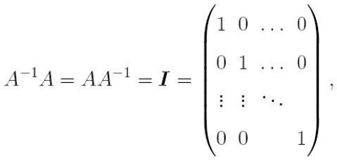
where I is the identity matrix.
We can write
![]()
This is done in MATLAB using the matrix inverse function (inv): x=inv(A)*b.
>> i=inv(A)*V
i =
17.0588
9.0784
-5.7843
7.9804
14.8627
Kramer’s formula:
>> DetA=det(A)
DetA =
-51
>> A1=[V A(:,2:end)]
A1 =
41 0 0 3 0
0 1 0 -3 1
38 0 -4 0 1
0 -1 0 -1 0
0 1 -1 0 -1
>> DetA1=det(A1)
DetA1 =
-870
>> A2=[A(:,1) V A(:,3:end)]
A2 =
1 41 0 3 0
0 0 0 -3 1
0 38 -4 0 1
1 0 0 -1 0
0 0 -1 0 -1
>> DetA2=det(A2)
DetA2 = -463
>> A3=[A(:,[1 2]) V A(:,[4 5])]
A3 =
1 0 41 3 0
0 1 0 -3 1
0 0 38 0 1
1 -1 0 -1 0
0 1 0 0 -1
>> DetA3=det(A3)
DetA3 =
295
>> A4=[A(:,1:3) V A(:,5)]
A4 =
1 0 0 41 0
0 1 0 0 1
0 0 -4 38 1
1 -1 0 0 0
0 1 -1 0 -1
>> DetA4=det(A4)
DetA4 = -407
>> A5=[A(:,1:end-1) V]
A5 =
1 0 0 3 41
0 1 0 -3 0
0 0 -4 0 38
1 -1 0 -1 0
0 1 -1 0 0
>> DetA5=det(A5)
DetA5 =
-7586.3.2
>> I(1)=DetA1/DetA;
>> I(2)=DetA2/DetA;
>> I(3)=DetA3/DetA;
>> I(4)=DetA4/DetA;
>> I(5)=DetA5/DetA;
>> I'
ans =
17.0588
9.0784
-5.7843
7.9804
14.8627
3.3.2 Iterative methods
Jacobi method
Let suppose that all diagonal elements aii i=1,2,…n, are nonzero. In this case we can write the system (3.1) in form:

 (3.5)
(3.5)
Let first approximation to solution(initial guess) of system is equal zero:
![]()
Let's
substitute these values in system of the equations (3.5)
and we shall receive the following approximation to the solution. In
common case, if we have calculated (k-1)-approximation
![]() we receive next approximation by formulas:
we receive next approximation by formulas:

 (3.6)
(3.6)
Repeating
iterations for k=1,2,… we receive the sequence of vectors (![]() ),
k=1,2,…
),
k=1,2,…
Theorem. If such conditions for diagonal elements aii , i=1,2,…n, hold:
![]()
or
![]() .
.
the repeated application of the method results in the appearance of the sequence tending to solution of system (3.1) as limit.
When the sequence converges, the difference between two next approximations to the decision tends to zero. Hence, we can believe, that have received the decision with the necessary accuracy, if distance between two approximations to the decision became less given accuracy .
Distance between two vectors can be measured by several various ways:
Distance is on the average calculated under the formula
![]()
Distance on the maximal value of coordinate of a vector is calculated under the formula:
![]()
Which of the formulas to use is decided depending on the requirements of practice.
Example. Solve system of linear equations using iterative method:
 4x1
– x2
+ x3
= 4
2x1 + 6x2 - x3 = 7
x1 +2x2 -3x3 = 0
First of all we shall check up, whether the conditions of convergence for a method of simple iterations are carried out. As 4>2, 6>3 and 33, the convergence condition are carried out and we can use this method.
L et's
express unknowns x1,
x2,
x3
accordingly from first, second and third equations:
x1 = (4 + x2 - x3 )/4
x2 = (7 - 2 x1 + x3 )/6
x3 = (x1 + 2 x2 )/3
It is easy to see that system has such solution: x1 =1, x2 =1, x3 =1.
As
a first approximation (as usually) let’s give
![]() Next
approximation we will receive if substitute these values in system of
the equations (3.7):
Next
approximation we will receive if substitute these values in system of
the equations (3.7):
![]()
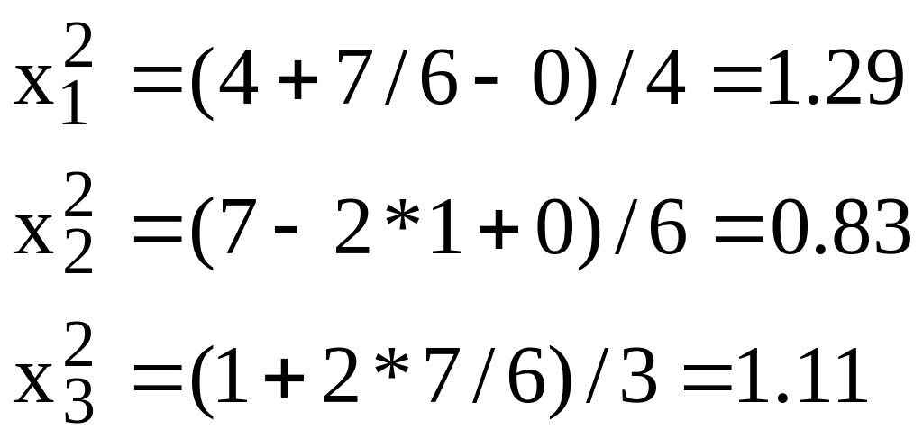
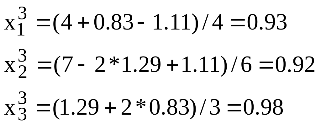
Next approximations are :

![]()
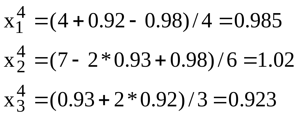
You see that unknowns tend to 1 – the solution of this system.
Listing of file jacobi.m. Solution of the linear system Ax = b, from the initial value of x = P0, and generating the sequence {Pk}, which converges to the solution. Effective conditions for the use of the method is that A - is strictly diagonally dominant matrix.
b is an n-by-1 known column vector; and x is an n-by-1 column vector of unknowns.
function [x,k]=jacobi(A,b,P,eps,maxiter)
%Input data:
% - A - non-singular matrix of size n * n,
% - b is an n-by-1 known column vector;
% - P is an n-by-1 column vector of initial guess,
% - eps - the variable that determines the accuracy
% of numerical solutions,
% - maxiter - maximum number of iterations.
%Output data:
% – x is an n-by-1 column vector of unknowns,
% - k number of iterations.
n=length(b);
for k=1:maxiter
for i=1:n
x(i)=(b(i)-A(i,[1:i-1,i+1:n])*P([1:i-1,i+1:n]))/A(i,i);
end
err=abs(norm(x’-P));
P=x’;
if err<eps
break;
end
end
x=x’;
Zadel’s method
This method differs from a method of simple iterations(Jacobi method) by that new calculated of approximation to the decision is immediately substituted in the equation for calculation of the following approximation. Thus, the calculations are made under the following formulas:

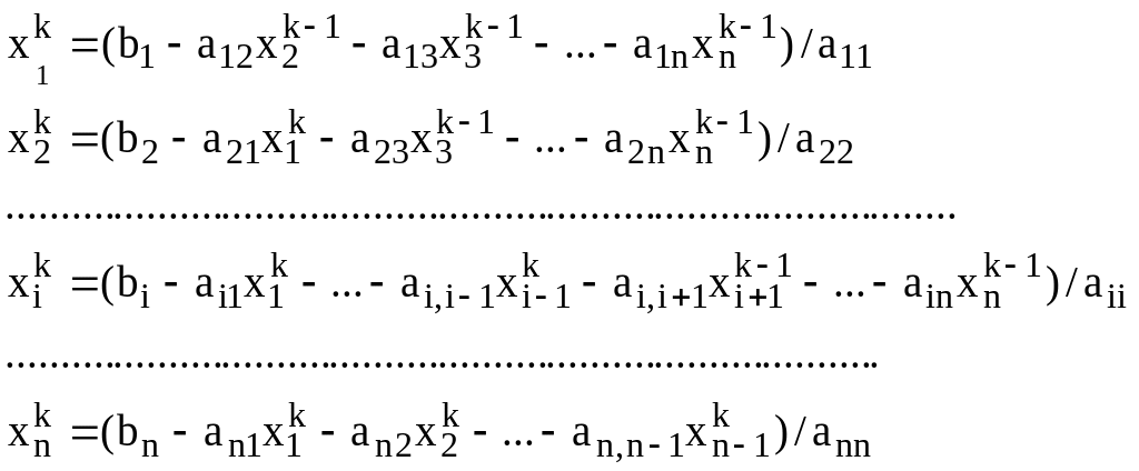 (3.9)
(3.9)
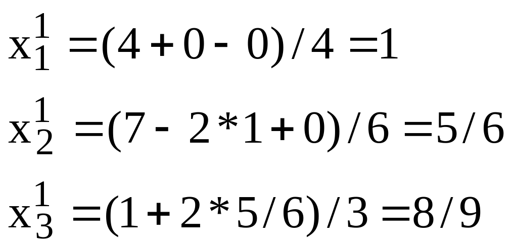
Example. Let’s find the solution of system from the previous example by Zadel’s method. As a first approximation (as usually) let’s give
By formulas (3.9) we receive:
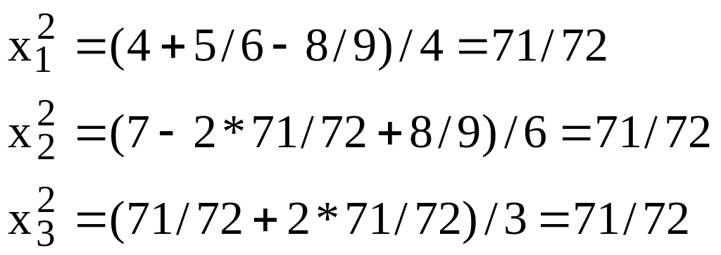
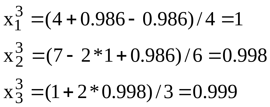
From this example you can see that method of Zadel tends to the solution of system more quickly than method of simple iterations.
