IlllIiij-

Table.7 the yearly records and equivalent fuzzy set.

Year	Al	A2	A3	A4	A5
1973	0	0	0	1	0.1
1974	0	0	0	1	0.5
1975	0	0.1	0.1	0.9	0
1976	0	0	0	1	0.9
1977	1	0.5	0.5	0	0
1978	0	0	0	0.7	1
1979	0	0.1	0.1	0.9	0
1980	0	0.8	0.8	0.2	0
1981	0	0	0	1	0.3
1982	0	0.4	0.4	0.6	0
1983	0	0.9	0.9	0.1	0
1984	0	0	0	1	0.9
1985	0	0.8	0.8	0.2	0
1986	0	0.4	0.4	0.6	0
1987	0	0	0	0.7	1
1988	0	0.3	0.3	0.7	0
1989	0	0.9	0.9	0.1	0
1990	0	0	0	0.7	1
1991	0.8	1	1	0	0

6. Construct the fuzzy forecasting model.

Let R(1) be the first fuzzy relational ^function, which can be written as

^{R(1)=F(1)T X} F(2) ⁽²⁴⁾

The elements of R(1) is defined as

r1=min(F(1)1, F(2)) ⁽²⁵⁾

^Where Y(1)1 represents ^{for the i-th element of Y(1), and for the j-th} elements of Y(2). For all the historical knowledge, the fuzzy relational functions are found and union operator is applied to obtained the model:

R=Union of R(i) (26)

4 kl41 rIrt I

^[P IJ1i

YTI

2. IL

14 t

^I J 1 1t

-

‘

In the case of ^n=5, R is a matrix of 5 ^X 5 whose values are as follows:

	o	o	0	0.7	1
	o	0.4	0.8	0.9	0.9
R=	0.1	0.9	1	1	1
	1	0.8	1	1	0.9
	0.9	1	1	0.9	0.1

^{7. Obtained forecasted} output ^data using ^R.

As the relational function is ^determined, historical data can be used to obtained the predicted values by

F(t)=F(t-1) R ⁽²⁷⁾

And the forecasted fuzzy sets in the case for n=5 are given in Table 8

Table.8 the forecasted fuzzy sets

Year	Membership					Normalized membership
1974	1	0.9	1	1	0.9	0.21	0.19	0.21	0.21	0.19
1975	1	0.8	1	1	0.9	0.21	0.17	0.21	0.21	0.19
1976	0.9	0.9	1	1	1	0.19	0.19	0.21	0.21	0.21
1977	1	0.9	1	1	0.9	0.21	0.19	0.21	0.21	0.19
1978	0	0.4	0.5	0.7	1	0	0.15	0.19	0.27	0.38
1979	00.9	1	1	0.9	0.7	0.2	0.22	0.22	0.2	0.16
1980	0.9	0.9	1	1	1	0.19	0.19	0.21	0.21	0.7
1981	0.2	0.9	1	1	1	0.05	0.22	0.24	0.24	1
1982	1	0.8	1	1	0.9	0.21	0.17	0.21	0.21	1
1983	0.6	0.9	1	1	1	0.13	0.2	0.22	0.22	0.7
1984	0.1	0.9	1	1	1	0.025	2.02	0.25	0.25	0.25
1985	1	0.9	1	1	0.9	0.21	0.19	0.21	0.21	0.19
1986	0.02	0.9	1	1	1	0.05	0.22	0.24	0.24	0.24
1987	0.6	0.9	1	1	1	0.013	0.2	0.22	0.22	0.22
1988	0.9	1	1	1	0.7	0.2	0.22	0.22	0.2	0.16
1989	0.7	0.9	1	0.9	1	0.15	0.2	0.22	0.22	0.22
1990	0.1	0.9	1	1	1	0.025	0.225	0.25	0.25	0.25
1991	0.9	1	1	1	0.7	0.2	0.22	0.22	0.2	0.16
1992	0.1	0.4	1	0.9	0.9	0.03	0.13	0.26	0.29	0.29

366

8. Transfer the output fuzzy set into forecasted records.

Since the output fuzzy ^results, they should be transfer into real numbers. The transferring process is called defuzzification [4,5]. The three-principle method [5

is used in this study.

100

10

50

-50

-100

-150

65 66 67 68 69 70 71 72 73 74 75 76 ‘77 78 79 80

YEAR

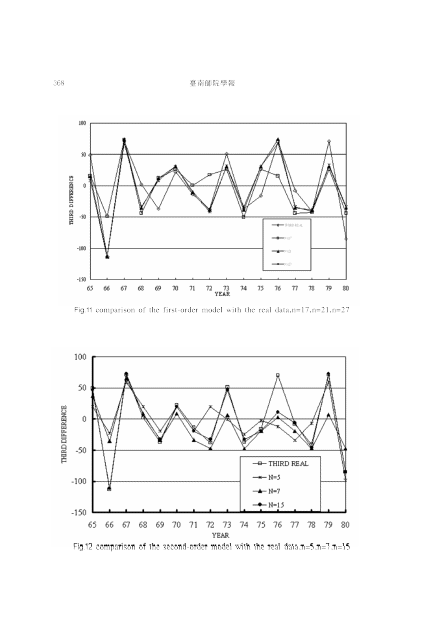
Fig.1O comparison of the first-order model with the real ^{data,n=5,n=7,n=15}

From the above ^{calculations,} it is found that the root mean square error is

0.119. Fig 10 shows the comparison of actual records and the current forecasted results.

For comparison, a second-order fuzzy time series model is developed for the same example. All the output fuzzy sets shown in Table 8 are ^useful, and they only serve as one of the possibility _F1 of the final output fLizzy sets for the

second-order model. Following the same processes, the second possibility of the

final output fuzzy sets _F12 are calculated as follows ^(Note that step 1- 4 are the same as the first-order model):

(5*) Setup the two-step-ahead fuzzy relations based on historical knowledge.

The first record in Table7 represents for the population in Taiwan area at ^1973, and the maximum membership is under _A4. ^Thus, we can view the first record as the linguistic _A4. When all the historical data are transferred into linguistic

expressions, the logical relations can be constructed. Note that a two-step-ahead

projection is applied instead of one-step-ahead projection used in step 5 of the first-order model.

(6*) Construct the two-step-ahead fuzzy forecasting model _R22.

Let R(1) be the first fuzzy relational ^function, which can be written as

367

_R22 ^{(1)=F(1)T X} F(3)

_R22 ^{(2)=F(2)T X} F(4) ⁽²⁸⁾

For example, the elements nj of _R22 (1) is defined as

r=min(F(1), F(3)) ⁽²⁹⁾

For all the historical knowledge, the two-step-ahead fLizzy relational functions are found and union operator is applied to obtained the two-step-ahead model:

^{R 2} _2=Union ^of R2(t) ⁽³⁰⁾

^(7*) Obtained the second possibility Ai2 using R22.

As the two-step-ahead relational function is ^determined, historical data can be used To obtained the predicted values by

F17=F(i-2) _R22 ⁽³¹⁾

^(8*) Take the intersection of _F11 and _F12 to form the output ^F(i).

Based on the proposed ^method, the essence of high-order time series models can be obtained while the simplicity of first-order calculation is retained. ^Furthermore, the formulation can be easily extended to higher-order models without any computational problems. The next section presents the application and comparisons of the results for the regression ^method, those for the first- and second-order models.

369

100

\

-100 ¹

-150

—S--THIRD REAL

—‘— ¹⁴⁼²¹

—*---N=27

65 66 67 68

Fig.13 comparison of the

69 70 71 72 73 74 75 76 77 78 79 80

YEAR

second-order model with the real ^data,n= 19^,n=2 1^,n=27

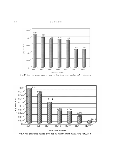
To reassure the effect of high-order ^model, the same example of the historical records of population in Taiwan area are analyzed using three different models ^(the regression ^method, the first and second-order ^models) with different numbers of fuzzy sets (n=5,7,15,19,21, and 27, where n represents for the number of fuzzy sets ). In Figs. ^11-13, the results obtained from the first-order and the second-order models are compared with the actual data for ^{n=5, 21,} and ^27, respectively. From these figures, the advantages of the proposed approach are clear. Better forecasting results are presented and the errors decrease for high values of n. This could be evidenced from Fig.14,l5, which shows the root mean square error obtained from forecasting models. The RMSE reduces from 0.17 for the regression method using the polynomial of degree

3 as shown in Fig.16, to 0.119 for the first-order model and 0.013 for the second-order model using n=27. This shows great improvement in forecasting results. The feasibility of the current formulation of the high-order fuzzy time series model is confirmed.

^p 4 t I J 1i^I J 1

[

rIrt I4 —I-’ TT1

_‘- Iu

1.6

R

M

S

E 0.8

0.6

04

0.2

^0.17 022 0.22

0.32