2. Classification of Real-Time Task Scheduling Algorithms

Several schemes of classification of real-time task scheduling algorithms exist. A popular scheme classifies the real­time task scheduling algorithms based on how the scheduling points are defined. The three main types of schedulers according to this classification scheme are: clock-driven, event-driven, and hybrid.

The clock-driven schedulers are those in which the scheduling points are determined by the interrupts received from a clock. In the event-driven ones, the scheduling points are defined by certain events which precludes clock interrupts. The hybrid ones use both clock interrupts as well as event occurrences to define their scheduling points.

A few important members of each of these three broad classes of scheduling algorithms are the following:

1. Clock Driven:

• Table-driven

• Cyclic

2. Event Driven:

• Simple priority-based

• Rate Monotonic Analysis (RMA)

• Earliest Deadline First (EDF)

3. Hybrid:

• Round-robin

Important members of clock-driven schedulers that we discuss in this text, are table-driven and cyclic schedulers. Clock-driven schedulers are simple and efficient,. Therefore, these are frequently used in embedded applications. We investigate these two schedulers in some detail in Sec. 2.4.

Important examples of event-driven schedulers are Earliest Deadline First (EDF) and Rate Monotonic Analysis (RMA). Event-driven schedulers are more sophisticated than clock-driven schedulers and usually are more proficient and flexible than clock-driven schedulers. These are more proficient because they can feasibly schedule some task sets which clock-driven schedulers cannot. These are more flexible because they can feasibly schedule sporadic and aperiodic tasks in addition to periodic tasks, whereas clock-driven schedulers can satisfactorily handle only periodic tasks. Event-driven scheduling of real-time tasks in a uniprocessor environment was a subject of intense research during early 1970’s, leading to publication of a large number of research results. Out of the large number of research results that were published, the following two popular algorithms are the essence of all those results: Earliest Dead­line First (EDF), and Rate Monotonic Analysis (RMA). If we understand these two schedulers well, we would get a good grip on real-time task scheduling on uniprocessors. Several variations to these two basic algorithms exist.

Another classification of real-time task scheduling algorithms can be made based upon the type of task acceptance test that a scheduler carries out before it takes up a task for scheduling. The acceptance test is used to decide whether a newly arrived task would at all be taken up for scheduling or be rejected. Based on the task acceptance test used, there are two broad categories of task schedulers:

• Planning-based

• Best effort

In planning-based schedulers, when a task arrives the scheduler first determines whether the task can meet its dead­lines, if it is taken up for execution. If not, it is rejected. If the task can meet its deadline and does not cause other already scheduled tasks to miss their respective deadlines, then the task is accepted for scheduling. Otherwise, it is rejected. In best effort schedulers, no acceptance test is applied. All tasks that arrive are taken up for scheduling and best effort is made to meet its deadlines. But, no guarantee is given as to whether a task’s deadline would be met.

A third type of classification of real-time tasks is based on the target platform on which the tasks are to be run. The different classes of scheduling algorithms according to this scheme are:

• Uniprocessor

• Multiprocessor

• Distributed

Uniprocessor scheduling algorithms are possibly the simplest of the three classes of algorithms. In contrast to unipro­cessor algorithms, in multiprocessor and distributed scheduling algorithms first a decision has to be made regarding which task needs to run on which processor and then these tasks are scheduled. In contrast to multiprocessors, the processors in a distributed system do not possess shared memory. Also in contrast to multiprocessors, there is no global uptodato state information available in distributed systems. This makes uniprocessor scheduling algorithms that assume a central state information of all tasks and processors to exist unsuitable for use in distributed systems. Further in distributed systems, the communication among tasks is through message passing. Communication through message passing is costly. This means that a scheduling algorithm should not incur too much communication over­head. So carefully designed distributed algorithms are normally considered suitable for use in a distributed system. We study multiprocessor and distributed scheduling algorithms in chapter 4.

In the following sections, we study the different classes of schedulers in more detail.

4. Clock-Driven Scheduling

Clock-driven schedulers make their scheduling decisions regarding which task to run next only at the clock interrupt points. Clock-driven schedulers are those for which the scheduling points are determined by timer interrupts. Clock- driven schedulers are also called off-line schedulers because these schedulers fix the schedule before the system starts to run. That is, the scheduler pre-determines which task will run when. Therefore, these schedulers incur very little run time overhead. However, a prominent shortcoming of this class of schedulers is that they can not satisfactorily handle aperiodic and sporadic tasks since the exact time of occurrence of these tasks can not be predicted. For this reason, this type of schedulers are also called a static scheduler.

In this section, we study the basic features of two important clock-driven schedulers: table-driven and cyclic schedulers.

1. Table-Driven Scheduling

Table-driven schedulers usually precompute which task would run when and store this schedule in a table at the time the system is designed or configured. Rather than automatic computation of the schedule by the scheduler, the application programmer can be given the freedom to select his own schedule for the set of tasks in the application and store the schedule in a table (called schedule table) to be used by the scheduler at run time.

An example of a schedule table is shown in Table. 1. Table 1 shows that task Ti would be taken up for execution at time instant 0, T-2 would start execution 3 milli seconds after wards, and so on. An important question that needs to be addressed at this point is what would be the size of the schedule table that would be required for some given set of periodic real-time tasks to be run on a system? An answer to this question can be given as follows: if a set ST={I;} of n tasks is to be scheduled, then the entries in the table will replicate themselves after LCM(pi ,ра,...,p_n) time units, where p\, pa,..., p_n are the periods of T\, ,.... For example, if we have the following three tasks: (c. \ =5

msocs, pi=20 msocs), (<°,₂=2Q msocs, р₂=100 msocs), (г?з=30 msocs, p?=250 msocs). Then, the schedule will repeat after every 500 msecs. So, for any given task set it is sufficient to store entries only for ЬСМ(р_1;р2, •••->Pn) duration in the schedule table. ЬСМ(р_1;р2, •••->Pn) is called the m,ajor cycle of the set of tasks ST.

A major cycle of a set of tasks is an interval of time on the time line such that in each major cycle, the different tasks recur identically.

In the reasoning we presented above for the computation of the size of a schedule table, one assumption that we implicitly made is that ф= 0. That is, all tasks are in phase.

Task	Start Time in milli Seconds
Tx	0
T-2	3
T3	10
Ti	12
n	17

Table. 1: An Example of a Table-Driven Schedule

However, tasks often do have non-zero phase. It would be interesting to determine what would be the major cycle when tasks have non-zero phase. The results of an investigation into this issue has been given as Theorem 2.1.

Theorem 2. 1. Th,e m,ajor cycle of a set of tasks ST={T\,T₂, ...,T_n } is LCM({pi,p-2,...,p_n}) even when the tasks have arbitrary phasings.

Proof: As per our definition of a major cycle, even when tasks have non-zero phasings, task instances would repeat the same way in each major cycle. Let us consider an example in which the occurrences of a task I; in a major cycle be as shown in Fig. 4. As shown in the example of Fig. 4, there are k-1 occurrences of the task I; during a major cycle. The first occurrence of I; starts ф time units from the start of the major cycle. The major cycle ends x time units after the last (i.e. (k-l)th) occurrence of the task I; in the major cycle. Of course, this must be the same in

Figure 4: Major Cycle When A Task Tj Has Non-Zero Phasing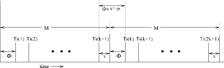

each major cycle.

Assume that the size of each major cycle is M. Then, from an inspection of Fig. 4, for the task to repeat identically in each major cycle.

M = (k — l)pt + ф + x ... (2.1)

Now, for the task T ^t0 have identical occurrence times in each major cycle, ф + х must equal to p.; (see Fig. 2.4).

Substituting this in Expr. 2.1 we get, M = (к — 1) *p* + p* = к *pi

So, the major cycle M contains an integral multiple of щ. This argument holds for each task in the task set

irrespective of its phase. Therefore, M=LCM({pi,p-2, ...,p_n}). □

2. Cyclic Schedulers

Cyclic schedulers are very popular and are being extensively used in the industry. A large majority of all small embedded applications being manufactured presently are based on cyclic schedulers. Cyclic schedulers are simple, efficient, and are easy to program. An example application where a cyclic scheduler is normally used is a temperature controller. A temperature controller periodically samples the temperature of a room and maintains it at a preset value. Such temperature controllers are embedded in typical computer-controlled air conditioners.

Task Number	Frame Number
T3	F1
T1	F2
T3	F3
T4	F2