

#38. What Can You Do about Autocorrelation?
Suppose that the model is Yt = β₁ + β₂Xt + ut (1), with ut generated by the process ut = ρu(t-1) + εt. If we lag first equation by one time period and multiply by ρ we will have ρY(t-1) = β₁ρ + β₂ρX(t-1) + ρu(t-1) (2). Now subtract (2) from (1). Yt – ρY(t-1) = β₁(1 – ρ) + β₂Xt - β₂ρX(t-1) + ut - ρu(t-1). Hence: Yt = β₁(1 – ρ) + ρY(t-1) + β₂Xt - β₂ρX(t-1) + εt. The model is now free from autocorrelation because the disturbance term has been reduced to the innovation εt.
#39. Multiple regression analysis. A Model with Two Explanatory Variables.
MRA is an extention of the SRA to cover causes in which the explained variable depends on more then one explanatory variable.
For example a true relationship may be expressed as EARNING = β₁ + β₂S + β₃ASVABC + u
S – years
ASVABC – composite score on the cognitive test in the Armed Services Aptitude
#40. Derivation of the Multiple Regression Coefficients. A Model with Two Explanatory Variables.
Let’s
assume that Y depends on 2 explanatory variables. As before our
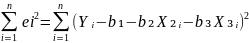
defenition of goodness of fit is the minimisation of RSS. RSS =

Where ei is the residuals in observation i.
Ŷi = b₁ + b₂X₂ᵢ + b₃X₃ᵢ
eᵢ = Yᵢ - Ŷᵢ = Yᵢ - b₁ - b₂X₂ᵢ - b₃X₃ᵢ
RSS
=
Firdt order condition for a minimum.
 =
-2
=
-2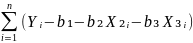 =
0
=
0
 =
-2
=
-2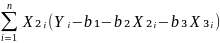 = 0
= 0
 =
-2
=
-2 = 0
= 0
b₁ = Ȳ - b₂X₂ - b₃X₃
b₂
=
b₃
=
#41. Derivation of the Multiple Regression Coefficients. The General Model.
Now we assume that Y depends on k-1 explanatory variables (X₁,...,Xk)
Yᵢ = β₁ + β₂X₂ᵢ + ... + βkXkᵢ +uᵢ true relationship.
Ŷᵢ = b₁ + b₂X₂ᵢ + ... + bkXkᵢ fitted line.
We will again minimize the the sum of squares of the residuals, which are given by:
eᵢ = Yᵢ - Ŷᵢ = Yᵢ - b₁ - b₂X₂ᵢ - ... - bkXkᵢ
We should choose b₁,...,bk so as to minimize RSS.
= 0
...
 =
0
=
0
The 1st of these equations yields: b₁ = Ȳ - b₂X₂ - ... – bkXk.
The expressions for b₂,...,bk become very complicated.
#42. Properties of the Multiple Regression Coefficients: Unbiasedness; Efficiency; Precision; Consistency.
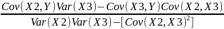
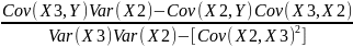
Unbiasedness. We may show that b₂ is an unbiased estimator of β₂ in the case where there are two explanatory variables.
∆ = Var(X₂)Var(X₃) – [Cov(X₂,X₃)²]
b₂
= ... =
 {Cov(X₂,|β₁
+ β₂X₂ + β₃X₃ + u|)Var(X₃) – Cov(X₃,|β₁ + β₂X₂
+ β₃X₃ +u|)Cov(X₂,X₃)} =
=
{[Cov(X₂,β₁)
+ Cov(X₂,β₂X₂) + Cov(X₂,β₃X₃) + Cov(X₂,u)]Var(X₃)
–
– [Cov(X₃,β₁) +
Cov(X₃,β₂X₂) + Cov(X₃,β₃X₃) + Cov(X₃,u)]Cov(X₂,X₃)}
=
=
{[β₂Var(X₂)
+ β₃Cov(X₃,X₂) + Cov(X₂,u)]Var(X₃) – [β₂Cov(X₃,X₂)
+ β₃Var(X₃) + Cov(X₃,u)]Cov(X₂,X₃)} =
=
{β₂Var(X₂)Var(X₃)
+ β₃Cov(X₃,X₂)Var(X₃) + Cov(X₂,u)Var(X₃) –
– β₂[Cov(X₂,X₃)²] –
β₃Var(X₃)Cov(X₂,X₃) – Cov(X₃,u)Cov(X₂,X₃)} =
=
{β₂(Var(X₂)Var(X₃)
– [Cov(X₂,X₃)²]) + Cov(X₂,u)Var(X₃) –
Cov(X₃,u)Cov(X₂,X₃)} =
=
{β₂∆
+ Cov(X₂,u)Var(X₃) – Cov(X₃,u)Cov(X₂,X₃)} =
= β₂ +
(Cov(X₂,u)Var(X₃)
– Cov(X₃,u)Cov(X₂,X₃)) = b₂
Thus b₂ has two components: the true value β₂ and an
error component. If we take the expectation we will obtain: E(b₂)
= β₂ +
Var(X₃)E[Cov(X₂,u)]
–
Cov(X₂,X₃)E(Cov(X₃,u))
Therefore
X₂ and X₃ are non stpchastic.
{Cov(X₂,|β₁
+ β₂X₂ + β₃X₃ + u|)Var(X₃) – Cov(X₃,|β₁ + β₂X₂
+ β₃X₃ +u|)Cov(X₂,X₃)} =
=
{[Cov(X₂,β₁)
+ Cov(X₂,β₂X₂) + Cov(X₂,β₃X₃) + Cov(X₂,u)]Var(X₃)
–
– [Cov(X₃,β₁) +
Cov(X₃,β₂X₂) + Cov(X₃,β₃X₃) + Cov(X₃,u)]Cov(X₂,X₃)}
=
=
{[β₂Var(X₂)
+ β₃Cov(X₃,X₂) + Cov(X₂,u)]Var(X₃) – [β₂Cov(X₃,X₂)
+ β₃Var(X₃) + Cov(X₃,u)]Cov(X₂,X₃)} =
=
{β₂Var(X₂)Var(X₃)
+ β₃Cov(X₃,X₂)Var(X₃) + Cov(X₂,u)Var(X₃) –
– β₂[Cov(X₂,X₃)²] –
β₃Var(X₃)Cov(X₂,X₃) – Cov(X₃,u)Cov(X₂,X₃)} =
=
{β₂(Var(X₂)Var(X₃)
– [Cov(X₂,X₃)²]) + Cov(X₂,u)Var(X₃) –
Cov(X₃,u)Cov(X₂,X₃)} =
=
{β₂∆
+ Cov(X₂,u)Var(X₃) – Cov(X₃,u)Cov(X₂,X₃)} =
= β₂ +
(Cov(X₂,u)Var(X₃)
– Cov(X₃,u)Cov(X₂,X₃)) = b₂
Thus b₂ has two components: the true value β₂ and an
error component. If we take the expectation we will obtain: E(b₂)
= β₂ +
Var(X₃)E[Cov(X₂,u)]
–
Cov(X₂,X₃)E(Cov(X₃,u))
Therefore
X₂ and X₃ are non stpchastic.
Efficiency.
The Gauss Markov theorem proves that for multiple regression analysis, the OLS technique yields the most efficient linear estimators.
In the sense tha it is impossible to find other unbiased estimators with lower variances using the same sample information provided that the Gauss Marov conditions are satisfied.
Precision.
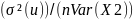
If
the true relationship is Yi = β₁ + β₂X₂ᵢ + β₃X₃ᵢ +
uᵢ andthe fitted line is Ŷi = b₁ + b₂X₂ᵢ + b₃X₃ᵢ
then we may find the population varience of the probability
distribution of b₂. Which is given by the formula: σ²(b₂) =
 *
*
Where is the population variance of u and r(X2X3) is the correlation
between X₂ and X₃. The statndard deviation of of the
distribution of b₂ is the square root of the variance. The
standard error of b₂ is the estimate of the standard deviation. So
we need to estimate
.
The biased estimator is E(Var(e)) =
is the population variance of u and r(X2X3) is the correlation
between X₂ and X₃. The statndard deviation of of the
distribution of b₂ is the square root of the variance. The
standard error of b₂ is the estimate of the standard deviation. So
we need to estimate
.
The biased estimator is E(Var(e)) =
 .
However we may obtain an unbiased estimator: S²𝗇
=
.
However we may obtain an unbiased estimator: S²𝗇
=
 Var(e)
The
standard error is given by the formula: s.e. =
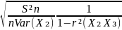 S𝗇
can be obtained directly from the regression output.
S𝗇
can be obtained directly from the regression output.
Sn²
is the sum of squares of the residuals devided by (n – k). Sn²
=
Var(e)
=
* =
= RSS
RSS
Consistency.
Provided that the Gauss Markov condition is satisfied, OLS yields consistent estimates in the multiple regression model.
As n becomes larger the population variance of the estimator of each regression coefficient tends to 0 and the collapses for a spike 1 condition for consistency.
Since the estimator is unbiased, the spike is located at the true value of the other condition for cnsistency.
#43. Multicollinearity.
In the case of a model with two explanatory variables: Ŷ = b₁ + b₂X₁ + b₃X₂ it was seen that the higher correlation between the explanatory variables – the large the population variances of the distribution of the coefficients and the greater is the risk of obtaining the erratic estimates of the coefficients. If the correlation causes the regression model to become unsatisfactory in this respect it is said to be suffering from multicollinearity.
#44. The Market Model.
This model assumes that the price of stock depends on the value of the market index. That’s why we may predict the future price of stock. In this model we take the stock price as Y and the market index as X and use simple regression to construct a fitted line. Then we use F test to verify the goodness of our model, T test to verify whether our coefficients are significant and which of them should be included in the model. Durbin Watson test to understand whether we have positive or negative auto correlation. Goldfeld Quandt test to learn whether our model is homo or heteroscedastic. If our model is good we may forecast the future price of stock.