Application Note

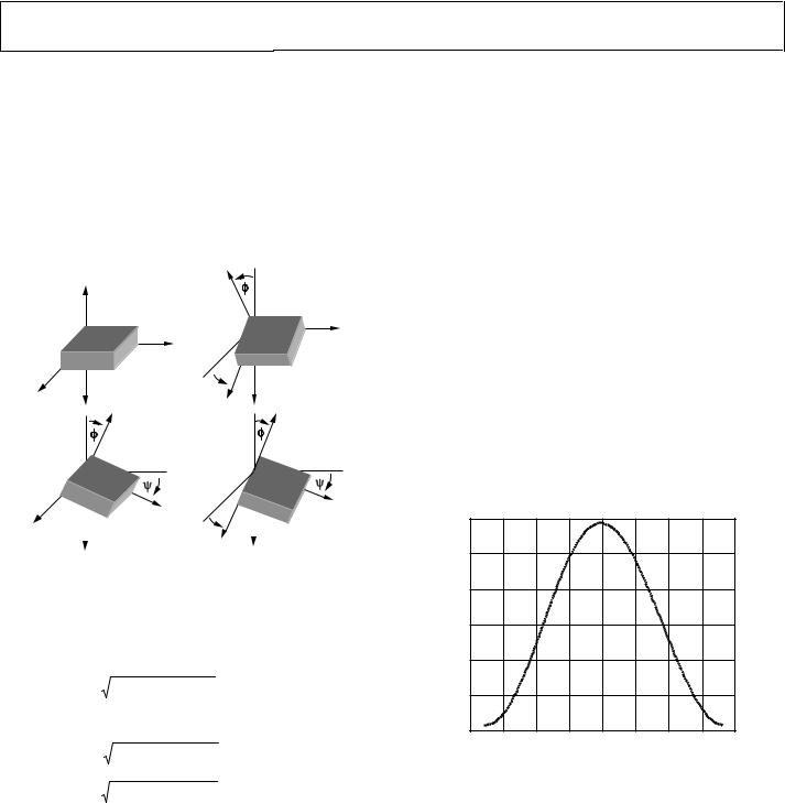
An alternative method for inclination sensing with three axes is to determine the angle individually for each axis of the accelerometer from a reference position. The reference position is taken as the typical orientation of a device with the x- and y-axes in the plane of the horizon (0 g field) and the z-axis orthogonal to the horizon (1 g field). This is shown in Figure 12 with θ as the angle between the horizon and the x-axis of the accelerometer, ψ as the angle between the horizon and the y-axis of the accelerometer, and

φ as the angle between the gravity vector and the z-axis. When in the initial position of 0 g on the x- and y-axes and 1 g on the z-axis, all calculated angles would be 0°.

Figure 12. Angles for Independent Inclination Sensing

Basic trigonometry can be used to show that the angles of inclination can be calculated using Equation 11, Equation 12, and Equation 13.

The apparent inversion of the operand in Equation 13 is due to the initial position being a 1 g field. If the horizon is desired as the reference for the z-axis, the operand can be inverted. A positive angle means that the corresponding positive axis of the accelerometer is pointed above the horizon, whereas a negative angle means that the axis is pointed below the horizon.

Because the inverse tangent function and a ratio of accelerations is used, the benefits mentioned in the dual-axis example apply, namely that the effective incremental sensitivity is constant and that the angles can be accurately measured for all points around the unit sphere.

AN-1057

CALIBRATION FOR OFFSET AND SENSITIVITY MISMATCH ERROR

The analysis in this application note was done under the assumption that an ideal accelerometer was used. This corresponds to a device with no 0 g offset and with perfect sensitivity (expressed as mV/g for an analog sensor or LSB/g for a digital sensor). Although sensors come trimmed, the devices are mechanical in nature, which means that any static stress on the part after assembly of the system may affect the offset and sensitivity. This, combined with the limits of factory calibration, can result in error beyond the allowable limits for the application.

Effects of Offset Error

To demonstrate how large the error can be, imagine first a dualaxis solution with perfect sensitivity but with a 50 mg offset on the x-axis. At 0° the x-axis reads 50 mg and the y-axis reads 1 g. The resulting calculated angle would be 2.9°, resulting in an error of 2.9°. At ±180° the x-axis would report 50 mg, whereas the y-axis would report −1 g. This would result in a calculated angle and error of −2.9°. The error between the calculated angle and the actual angle is shown in Figure 13 for this example. The error due to an offset may not only be large compared to the desired accuracy of the system, but it can vary, thus making it difficult to simply calibrate out an error angle. This becomes more complicated when an offset for multiple axes is included.

Figure 13. Calculated Angle Error Due to Accelerometer Offset

Effects of Sensitivity Mismatch Error

The main error component due to accelerometer sensitivity in a dual-axis inclination sensing application is when a difference in sensitivity exists between the axes of interest (as opposed to a single-axis solution, where any deviation between the actual sensitivity and the expected sensitivity results in an error).

Because the ratio of the x- and y-axes is used, most of the error is cancelled if the sensitivities are the same.

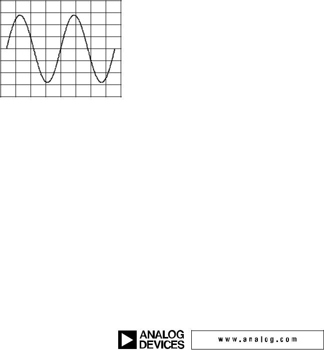
As an example of the effect of accelerometer sensitivity mismatch, assume that a dual-axis solution is used with perfect offset trim, perfect sensitivity on the y-axis, and +5% sensitivity on the x-axis. This means that in a 1 g field, the y-axis reports 1 g, whereas the x-axis reports 1.05 g. Figure 14 shows the error in the calculated angle due to this sensitivity mismatch. Similar to offset error, the error due to accelerometer sensitivity mismatch varies over the entire range of rotation, making it difficult to compensate for the error after calculation of the inclination angle. Skewing the mismatch further by varying the y-axis sensitivity results in even greater error.

Figure 14. Calculated Angle Error Due to Accelerometer Sensitivity Mismatch

Basic Calibration Techniques

When the errors due to offset and sensitivity mismatch are combined, the error can become quite large and well beyond the acceptable limits in an inclination sensing application. To reduce this error, the offset and sensitivity should be calibrated and the calibrated output acceleration used to calculate the angle of inclination. When including the effects of offset and sensitivity, the accelerometer output is as follows:

where:

AOFF is the offset error, in g.

Gain is the gain of the accelerometer, ideally a value of 1. AACTUAL is the real acceleration acting on the accelerometer and the desired value, in g.

©2010 Analog Devices, Inc. All rights reserved. Trademarks and registered trademarks are the property of their respective owners.

AN08767-0-2/10(0)

A simple calibration method is to assume that the gain is 1 and to measure the offset. This calibration then limits the accuracy of the system to the uncalibrated error in sensitivity. The simple calibration method can be done by placing the axis of interest into a 0 g field and measuring the output, which would be equal to the offset. That value should then be subtracted from the output of the accelerometer before processing the signal. This is often referred to as a no-turn or single-point calibration, because the typical orientation of a device puts the x- and y-axes in a 0 g field. If a three-axis device is used, at least one turn or a second point should be included for the z-axis.

A more accurate calibration method is to use two points per axis of interest (up to six points for a three-axis design). When an axis is placed into a +1 g and −1 g field, the measured outputs are as follows:

where the +1 g and −1 g measurements, A+1g and A−1g, are in g.

This type of calibration also helps to minimize cross-axis sensitivity effects as the orthogonal axes are in a 0 g field when making the measurements for the axis of interest. These values would be used by first subtracting the offset from the accelerometer measurement and then dividing the result by the gain.

where AOUT and AOFF are in g.

The calculations of AOFF and Gain in Equation 15 through Equation 19 assume that the acceleration values, A+1g and A−1g, are in g. If acceleration in mg is used, the calculation of AOFF in Equation 17 remains unchanged, but the calculation of Gain in Equation 18 should be divided by 1000 to account for the change in units.