AN-1057

Because the output of the accelerometer obeys a sinusoidal relationship as it is rotated through gravity, conversion from acceleration to angle is done using the inverse sine function.

where the inclination angle, θ, is in radians.

If a narrow range of inclination is required, a linear approximation can be used in place of the inverse sine function. The linear approximation relates to the approximation of sine for small angles.

where the inclination angle, θ, is in radians.

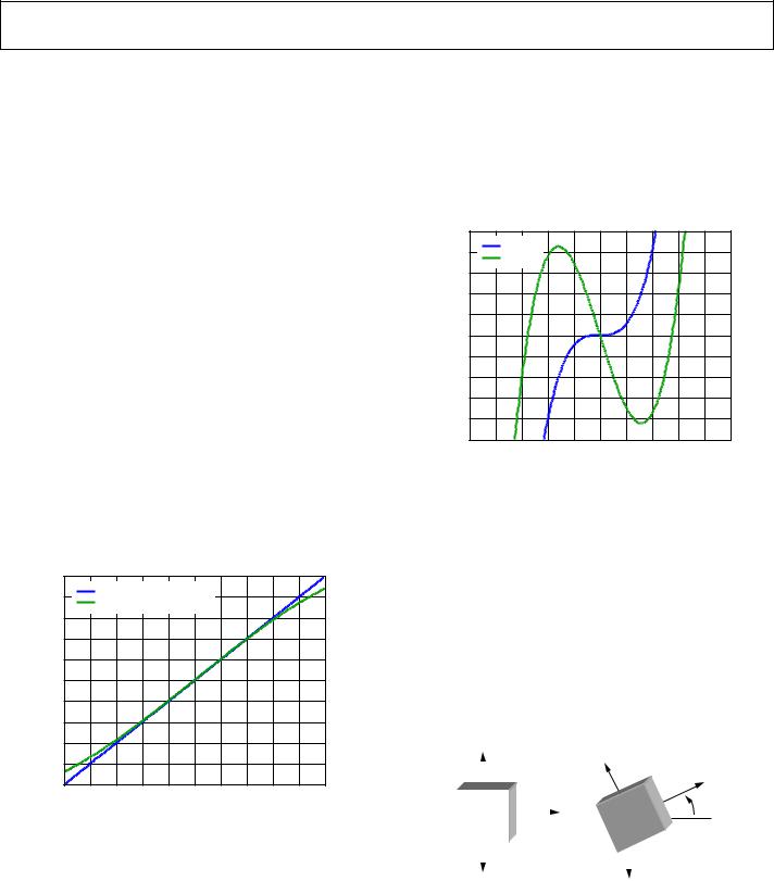
Conversion to degrees is done by multiplying the result of Equation 5 by (180/π). Figure 5 shows a comparison between using the inverse sine function and the linear approximation with k equal to 1. As the magnitude of the inclination angle increases, the linear approximation begins to fail, and the calculated angle deviates from the actual angle.

Figure 5. Comparison of Inverse Sine Function and Linear Approximation for Inclination Angle Calculation

Because the calculated angle is plotted against the actual angle of inclination, the linear approximation appears to bend near the ends. This is because the linear approximation is linear only when compared to the output acceleration and, as shown in Figure 2, the output acceleration behaves similarly as the actual angle of inclination is increased. However, the inverse sine function should produce an output that is one-to-one with the actual angle of inclination, causing the calculated angle to be a straight line when plotted against the actual angle of inclination.

Application Note

As an example, if the desired resolution of inclination sensing is 1°, an error of ±0.5° is acceptable because it is below the rounding error of the calculation. If the error between the actual angle of inclination and the calculated angle of inclination is plotted for k equal to 1, as shown in Figure 6, the valid range for the linear approximation is only ±20°. If the scaling factor is adjusted such that the error is maximized but kept within the calculation rounding limits, the valid range of the linear approximation increases to greater than ±30°.

Figure 6. Calculated Angle Error for Different Scaling Factors

Dual-Axis Tilt Calculation

One limitation of single-axis inclination sensing is the need for a high resolution ADC or digital output to achieve a large range of valid inclination angles, as shown in Figure 3 and Figure 4.

Another limitation is that a single-axis measurement cannot provide a 360° measurement, because the acceleration generated at an inclination of N° is the same as the acceleration generated at an inclination of 180° − N°. For some applications, this is acceptable, but for applications that require higher resolution or the ability to distinguish angles of inclination in a complete 360° arc, a second axis, as shown in Figure 7, or a second sensor is necessary. If a second sensor is used, it should be oriented such that the sensing axis of the second sensor is orthogonal to the sensing axis of the first sensor.

Figure 7. Two Axes Used for Tilt Sensing

There are three major benefits to including a second axis in determining the angle of inclination. These benefits are described in the following sections.

Application Note

Constant Sensitivity

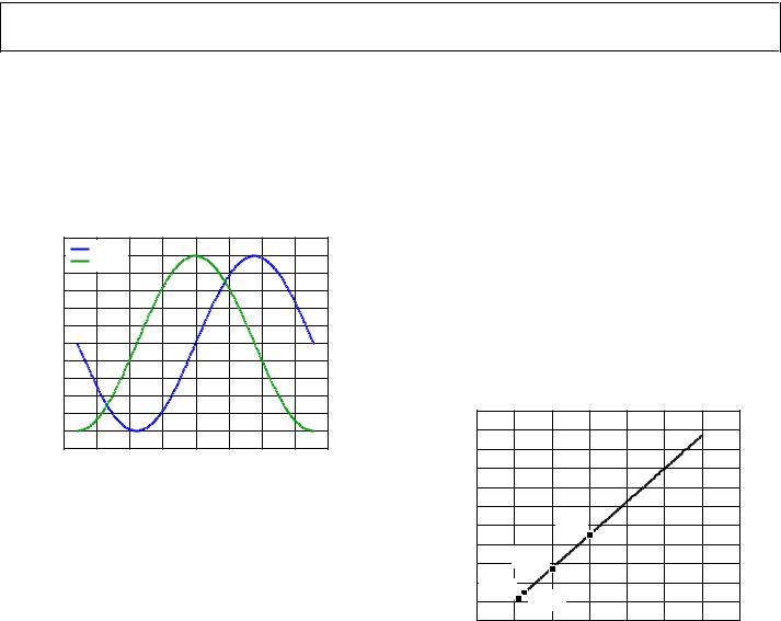
The first major benefit of using a second axis is due to the orthogonality of the axes. As in the single-axis solution, the acceleration detected by the x-axis is proportional to the sine of the angle of inclination. The y-axis acceleration, due to the orthogonality, is proportional to the cosine of the angle of inclination (see Figure 8). As the incremental sensitivity of one axis is reduced, such as when the acceleration on that axis approaches +1 g or −1 g, the incremental sensitivity of the other axis increases.

Figure 8. Output Acceleration vs. Angle of Inclination for Dual-Axis Inclination Sensing

One method to convert the measured acceleration to an inclination angle is to compute the inverse sine of the x-axis and the inverse cosine of the y-axis, similar to the single-axis solution. However, an easier and more efficient approach is to use the ratio of the two values, which results in the following:

where the inclination angle, θ, is in radians.

Unlike the single-axis example, using the ratio of the two axes to determine the angle of inclination makes determining an incremental sensitivity very difficult. Instead, it is more useful to determine the minimum necessary accelerometer resolution, given a desired inclination resolution. Given that the incremental sensitivity of one axis increases as the other decreases, the net result is an effective incremental sensitivity that is roughly constant. This means that the selection of an accelerometer with sufficient resolution to achieve the desired inclination step size at one angle is sufficient for all angles.

To determine the minimum necessary accelerometer resolution, Equation 6 is examined to determine where the resolution limitations are. Because the output of each axis relies on the sine or cosine of the angle of inclination, and the angle of inclination for each function is the same, the minimum resolvable angle corresponds to the minimum resolvable acceleration.

AN-1057

As shown in Figure 3 and Figure 4, the sine function has the greatest rate of change near 0°, and it can be shown that the cosine function has the least rate of change at this point. For this reason, the change in acceleration on the x-axis due to a change in inclination is recognized before a change in acceleration on the y-axis. Therefore, the resolution of the system near

0° depends primarily on the resolution of the x-axis. To detect an inclination change of P°, the accelerometer must be able to detect a change of approximately

Figure 9 can be used to determine the minimum necessary accelerometer resolution—or maximum accelerometer scale factor—for a desired inclination step size. Note that increased accelerometer resolution corresponds with a reduction in accelerometer scale factor and with the ability to detect a smaller change in output acceleration. Therefore, when selecting an accelerometer with the appropriate resolution, the scale factor should be less than the limit shown in Figure 9 for the intended inclination step size.

Figure 9. Minimum Accelerometer Resolution for a Desired Angle of Inclination Resolution

Reduced Dependence on Alignment with Plane of Gravity

The second major benefit of using at least two axes is that unlike the single-axis solution, where tilt in any axis other than the x-axis can cause significant error, the use of a second axis allows for an accurate value to be measured even when inclination in the third axis is present. This is because the effective incremental sensitivity is proportional to the root-sum-square (RSS) value of gravity on the axes of interest.

When gravity is completely contained in the xy-plane, the RSS value of acceleration detected on those axes is ideally equal to 1 g. If tilt is present in the xzor yz-plane, the total acceleration due to gravity is reduced, which also reduces the effective incremental sensitivity. This, in turn, increases the inclination step size for a given accelerometer resolution, but still provides an accurate measurement. The resulting angle from the inclination calculation corresponds to the rotation in the xy-plane.