диафрагмированные волноводные фильтры / d0b6eab4-ee66-48f9-8028-3068c251b6eb

This type of radar is commonly used for traffic regulation. The speed indicator used by the policemen is a kind of CW radar. The frequency shift fd is proportional to oscillation frequency f0 and the relative velocity of the target r.

The graph of Doppler frequency as a function of oscillation frequency and some relative target velocities calculated using MATLAB 6.5 is given in Appendix B. An interesting example of the CW radar is the proximity fuze widely used during World War II. This fuze is one of the first examples of the proximity fuzes which operate by the principles of radar.

2.4.3 Frequency Modulated Continuous Wave (FMCW)

Radar

Frequency Modulated Continuous Wave (FMCW) radar is a kind of continuous wave radar. Continuous wave radars are unable to measure the distance between radar and target. To measure the distance a sort of timing signal must be applied to the continuous wave carrier. In the FMCW radar the timing mark can be achieved by frequency modulating the continuous wave carrier. The changing frequency acts as a time marker and the elapsed time between transmission and the receiving the reflected wave can be calculated from the difference in frequency of the reflected signal and the transmitter. Another advantage of the FMCW radar system is simplicity of design when compared to a pulsed radar system. Block diagram of a typical FMCW radar system may be seen in Figure (2.5).

12

Receiving

antenna

Figure 2.5 FMCW radar system

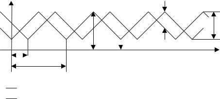
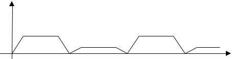
In FMCW radar systems the common frequency source is a voltage controlled oscillator (VCO). The modulation frequency cannot increase continually and must be periodic, thus VCO is usually controlled by a sawtooth wave shape generator. When the VCO is controlled by sawtooth wave shape generator the characteristics of the modulated signal may be seen in Figure (2.6). In Figure (2.6);

fm = 1 / Tm = Modulation frequency, fmax – fmin = f = Frequency deviation, Td = Delay time.

The frequency difference between the transmitted signal and the received signal indicates the distance between radar and the target. This frequency is the major identifier for distance measurement and called the beat frequency (fb). The beat frequency fb, is the indicator of the distance between radar and target. For amplitude fluctuations the beat frequency is amplified by a low frequency amplifier and then limited by a limiter. The distance R can be calculated from Equation (2.11).

13

f

fb

f

fmax

fmin

Tm

Frequency of transmitted signal

Frequency of received signal

Figure 2.6 Frequency variation of transmitted and received signal

In Equation (2.11), fm is the modulation frequency and c is the speed of light where f is the deviation of the modulation frequency which is the difference between the maximum and the minimum frequency of the transmitted signal.

m

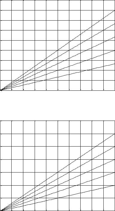
The greater the deviation of the transmitted signal in a given time interval, the more accurate the transit time (Td) can be measured and this result a greater transmitted spectrum. Speed of light, modulation frequency (fm) and the deviation of the modulation frequency ( f) is assumed to be constant, thus the distance from radar to the target is a function of the beat frequency (fb). For some different values of frequency deviation and modulation frequency, beat frequency versus distance from radar to target is given in Figure (2.7) and Figure (2.8).

14

Beat Frequency (KHz)

Distance (m.)

Figure 2.7 Beat frequency variation (fm = 1 KHz)

Beat Frequency (KHz)

Distance (m.)

Figure 2.8 Beat frequency variation (fm = 3 KHz)

15

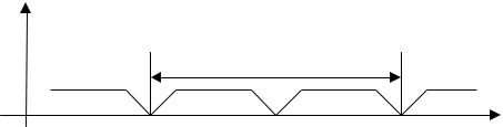
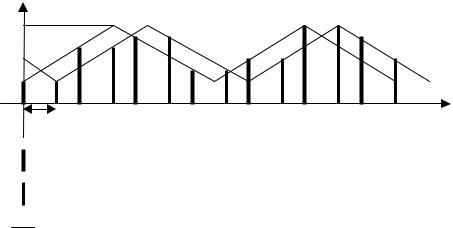
The choice of frequency modulation and modulation deviation is determined by the ranging sensitivity, K = 4fm f / c (Hz/m). For example if a VCO is linearly modulated at a rate of 10 KHz per over a range of 1 GHz the beat frequency of the FMCW system will be 133 KHz per meter of range. A wider range of frequencies swept by the modulation waveform and a higher frequency of the modulating waveform will yield more accurate measurement of the range information. Another consideration for beat frequency and doppler shift must be made if the radar or the target is in motion. A frequency shift by doppler effect will be superimposed on the beat note and an erroneous range measurement results. The doppler frequency shift will causes the beat frequency echo signal to be shifted up or down by doppler shift (fd). Figure (2.9) illustrates the beat frequency time plot of the echo signal. On the time plot of the beat frequency the doppler shift can be seen in Figure (2.10).

fb

Tm

fb

t

Figure 2.9 Beat frequency variation in time (for stationary objects)

16

fb

fb + fd

fb - fd

t

Figure 2.10 Beat frequency variation in time (for moving objects)

The doppler shift resulting from the moving platforms will yield smaller doppler shift compared to beat frequency. Assume that the FMCW radar frequency is around 850 MHz with modulation frequency (fm) is 3 KHz and modulation deviation ( f) is 30 MHz. The beat frequency for a target at a distance of 1000 meters is

and if the target is moving towards the radar with a radial velocity of 500 km/h (139 m/s) the doppler shift of the received frequency is only

The frequency shift due to doppler effect is only 787.67 Hz whilst the beat frequency is 1.2 MHz. When designing FMCW radar this doppler shift in this example can be neglected regarding to the application area and the design frequencies of the radar. If the target is in motion and the beat signal contains a component due to doppler frequency shift, the range frequency (fb-fd) can be extracted from the received signal. The achieve the range frequency, average of the beat signal frequency is measured and the modulation waveform

17

must have equal upsweep and downsweep regarding the doppler frequency shift. Also when the average of the beat frequency is measured for one cycle of the modulation frequency, the doppler effect will be cancelled.

2.4.4Pulse Modulated FMCW Radar

Another type of the FMCW radar is the pulse modulated FMCW radar. In the pulse modulated FMCW radar, the transmitter transmits the signal only for a limited time interval and then the receiver listen for the echoes of the transmitted signal.

In pulse modulated FMCW radar the transmitted signal reflects back from the target and the frequency of the received signal compared with the modulator frequency. Beat frequency is the difference between the modulator frequency and the received signal. The modulator frequency acts as a time marker as in the FMCW radar. Except from the FMCW radar the pulse modulated radar has blind range. Blind range occurs when the signal pulse is transmitted because the receiver is blocked within the time period of transmission.

Transmitted signal (pulse)

Received signal (echo of the pulsed signal)

Modulation waveshape

Figure 2.11 Pulse modulated FMCW radar frequency variation

18

Despite the range limitation of the pulse radar that is

limited to a value depending on the unambiguous distance (Runamb) given in Equation (2.8), the pulse modulated FMCW does not have range ambiguities depending on the pulse repetition frequency. Because pulse modulated FMCW radar

utilizes the beat frequency measurement instead of time

delay measurement. The blind range (Rp) is calculated from Equation (2.12) and the multiples of the blind range are also blind. Tp is the pulse interval.

The blind range width is dependant to the pulse width of the transmitted pulse. It is advantageous to reduce the pulse

width as short as possible to achieve the minimal blind

range width. Actually, FMCW radar also has range ambiguities and maximum range depending to the modulation frequency. The maximum range (Rmax) is equal to the distance traveled by a wave (velocity = speed of light) within the half period of the frequency modulation. For example, if the modulation

frequency is 1 KHz then the maximum unambiguous distance is

Tm/2 times the speed of light. If this is the case maximum unambiguous distance is 149.897 kilometers. If the distance

exceeds the maximum distance (2Rmax>R>Rmax) the calculated beat frequency peak will be

Equation (2.13) results from the downsweeping of the triangular waveform. When the distance (R) is longer from the maximum distance (Rmax) the modulation frequency slope changes its sign from positive to negative or vice versa after the delay time (td) corresponding to distance of the

19

target. This theoretical result does not occur because the maximum distance is usually much longer from the target distance at the FMCW radar applications. If the modulation frequency fm is equal to 3 KHz, the maximum distance Rmax will be 100 kilometers. And if the target distance is longer than 100 km then we can easily change the modulation frequency to a higher value then 3 KHz and these situations are usually well defined at the design phase.

20

CHAPTER 3

SURFACE ACOUSTIC WAVE (SAW) DEVICES

3.1Introduction to SAW Devices

Integrated Circuits (IC) are small and contain many elements up to 108. At the same time it is important that

ICs contain only transistors, diodes, resistors and

capacitors. Practically inductive elements cannot be integrated in monolithic ICs.

With the development of ICs, the problem of miniaturization of filters, delay lines and other components that included inductive elements appeared. As a result of search of ways to miniaturize mentioned components, surface

acoustic wave (SAW) devices were created.

The fundamentals of this technique lie in the

discovery of the piezoelectricity by the brother Curie in 1880 and of the surface acoustic waves in 1885 which is the

basis of the SAW devices by the famous English scientist

Lord Rayleigh. Piezoelectricity is a coupling between

elastic deformation and electric polarization which exists

in certain crystals such as quartz. Surface waves are piezoelectric microwaves which can be propagated over the surface of these crystals at a velocity of the order 3500 m/s. After the studies of Rayleigh, the surface acoustic waves are first observed at the beginning of the twentieth century that an earthquake could be detected at a great distance by two tremors corresponding to the modes of volume