Добавил:

ivanov666 Опубликованный материал нарушает ваши авторские права? Сообщите нам.

Вуз:

Башкирский Государственный Аграрный Университет

Предмет:

[НЕСОРТИРОВАННОЕ]

Файл:

книги2 / MK-1670

.pdf

Скачиваний:

Добавлен:

24.02.2024

Размер:

6.1 Mб

Скачать

☆

<<< < Предыдущая 1 2 3 4 5 67 / 297 8 9 10 11 12 13 14 15 16 17 18 19 20 21 22 23 24 25 > Следующая >>>

МОЛОДЁЖЬ, НАУКА, ОБРАЗОВАНИЕ 61

quantitative change in relative displacements, and, consequently, shear stresses in these sections.

Changes in stresses over time in fixed sections of the pipeline x = 5; 10; 15; 20; 25, and 30 m, obtained

in calculations, showed that, compared with the case when

	2

1.1

, a qualitatively different pattern is ob-

served. In this case, the stress amplitudes in the pipeline sections x=5;10;15, and 20m grow all the time and become steady in section x=25m.

Quantitatively, they differ by approximately 1.25 times from the case when 2

1.1

. An increase in

the maximum stress values in the pipeline sections for 2 2 , is a consequence of an increase in the soil

deformability. The process of steadying the maximum stress value, with a decrease in soil stiffness, increases. In this case, it is seen that the increase in the values of longitudinal stresses in the sections of the pipeline does not occur indefinitely.

Stresses in the same sections of the pipeline x = 5; 10; 15; 20, and 30 m for the case when

	2

, in-

creases, tends to a steady state and in section x = 30 m reaches the value of 165 MPa. This is 1.7 times more

than the values obtained for

	2

1.1

(70%), and 1.35 more than for

	2	2
	2

(35%). These results indicate

that when the soil surrounding the pipeline is soft (not compacted, the pipeline increase significantly. In the case of compacted soil (

	2
	2

2

4 ), the values of longitudinal stress in

1.1, Fig. 1), the stress values are 1.7

times lower.

The results of estimating the values of longitudinal stresses in underground gas pipelines during the Gazli earthquake are given in [6]. According to [6], the maximum values of longitudinal stresses for main underground pipelines are 1max (36.5 85) MPa.

Based on this, we can say that the calculated values of longitudinal stresses obtained in Fig. 1 are 12% higher than the upper limit of stresses observed in pipelines during earthquakes. This confirms the correctness of the calculation results obtained in the study.

The calculation results show that an account for the strain characteristics of soil leads to new qualitative and quantitative results. In this article, we considered the effect of a plane longitudinal seismic wave at a frequency of 0.05 s-1 on an underground pipeline. The results of the calculations showed that with an increase in the frequency of seismic waves, the maximum value of the longitudinal stresses in the underground pipeline decreases.

CONCLUSION

The results obtained are the scientific basis for improving the technology of underground pipeline construction. To increase the seismic resistance of underground pipelines, it is necessary to increase the soil density and the cohesion force of soil surrounding the pipeline. Consequently, the stiffness (strength) of soil increases, and the relative displacement decreases, which ensures the formation of relatively low longitudinal stresses in the pipeline. This leads to a decrease in the probability of failure in underground pipelines being built in earthquake-prone regions.

References

1.L.V. Nikitin // Statics and dynamics of solids with external dry friction. Moscow: 1998. 261 p.

2.K.S. Sultanov // Wave theory of seismic resistance of underground structures. Tashkent: Fan, 2016. 392 p.

3.K.S. Sultanov, N.I. Vatin, // Wave Theory of Seismic Resistance of Underground Pipelines. Applied Sciences. 2021. No. 4. Pp. 1797.

4.K.S. Sultanov, A.A. Bakhodirov // Laws of shear interaction on contact surfaces of rigid bodies with soils. OFMG. 2016. No. 2. P. 5-10.

5.K.S. Sultanov // Parameters of nonlinear laws of interaction of underground pipelines with soil. OFMG, No. 4, 2022. P.13-18.

6.K.S. Sultanov, J.X. Kumakov, P.V. Loginov, B.B. Rikhsieva // Strength of underground pipelines

VII International scientific conference | www.naukaip.ru

62 МОЛОДЁЖЬ, НАУКА, ОБРАЗОВАНИЕ

under seismic effects. Magazine of Civil Engineering. 2020.93(1). pp. 97-120.

7. A.A. Bakhodirov, K.S. Sultanov // Waves in a viscoelastic rod surrounded by a soil medium under smooth loading. MTT. 2014. No. 3. P. 132-144.

VII международная научно-практическая конференция | МЦНС «НАУКА И ПРОСВЕЩЕНИЕ»

МОЛОДЁЖЬ, НАУКА, ОБРАЗОВАНИЕ 63

UDC 62

SIMULATION OF BEHAVIOR OF UNDERGROUND PIPELINE WITH SOIL UNDER SEISMIC IMPACT

Akbarov Nodirbek Askaraliyevich

PhD student Institute of Mechanics and Seismic Stability of Structures named after M.T.Urazbaev AS RUz

Abstract. The paper presents a numerical solution to the problem of determining the longitudinal stresses in underground elastic pipelines, taking into account the wave theory (a one-dimensional statement) and the stiffness of the surrounding soil.

Key words: underground pipeline, soil, seismic waves, stresses, finite difference method, characteristic method.

INTRODUCTION

The problem of ensuring the seismic resistance of underground pipelines is related to the technology of their construction. Underground pipelines are divided into various types according to their purpose. This article will focus on the main underground pipelines [1-4].

The purpose of this study is to determine the effect of mechanical characteristics of soil surrounding an underground pipeline on the seismic strength of the pipeline and to improve the technologies of their construction that provide the required soil characteristics after construction.

SUBJECT AND METHODS OF RESEARCH

To achieve this goal, it is necessary to consider the influence of mechanical characteristics of soil surrounding the underground pipeline on the stress state of the pipeline since the assessment of seismic resistance of underground pipelines is somehow reduced to the determination of stresses in the body of the pipe by various methods [7]. The stress state of an underground pipe under the impact of seismic forces is quite complex [5]. For simplicity, the stresses are divided into longitudinal (along the axis of the pipeline), transverse (perpendicular to the axis of the pipeline), bending, radial, circular, and other [2-5]. Many authors noted that the most dangerous are longitudinal stresses [3, 4]. The subject of the study is the stress state of an underground pipeline under longitudinal seismic impacts.

According to the wave theory of seismic resistance of underground structures [5], the force that creates a stress state in an underground pipeline is the interaction force between the pipeline and soil under seismic impacts. This force directly depends on the degree of soil strain around the pipeline. Therefore, in wave theory, it is considered important to determine the stress-strain state of soil under the impact of seismic load.

Considering the above, the system of equations in wave theory, which describes the process of interaction of an underground pipeline with soil under the action of seismic loads in the case of a one-dimensional motion for soil, has the following form:

VII International scientific conference | www.naukaip.ru

64 МОЛОДЁЖЬ, НАУКА, ОБРАЗОВАНИЕ

0 g

EDg t

ESg

(1)


where	0 g	is the initial density of soil,		v	g	is the particle velocity (mass velocity) of soil,	g	is the longitudi-

nal stress (along the			x -axis ) in soil,	g		is the reduced force of the interaction of the underground pipeline

with soil,

is the longitudinal strain (along the x-axis) of soil,

is the volumetric viscosity parameter of

soil,

g is the coefficient of volumetric viscosity of soil,

is the dynamic modulus of soil compression as

the

static modulus

soil

compression

dt 0

is the spatial coordinate

(along the axis of the pipeline), t is time.

The values of

g and

are determined by the following relations:

(2)

N NS

(3)

g H c DH2

DB2

4DH

(4)

K g

(5)

sgn

v v

(6)

where

is the depth of laying of the pipeline in soil,

is the outer diameter of the underground pipeline,

is the unit weight of soil,

c is the unit weight of the pipeline material,

is the lateral pressure coeffi-

cient in soil, v

is the relative velocity,

is the velocity of the soil particles,

is the velocity of the pipeline

sections,

is the static soil stress normal to external surface,

is the dynamic stress normal to the ex-

ternal surface of soil.

The equations of motion, continuity, and strain of an underground pipeline have the following form:

(7)

c ESc

EDc t

EDc ESc

where 0c is

the initial density of the pipeline material, c

is the longitudinal stress (along the axis of the

pipeline) in the pipeline, c

is the reduced force of interaction (friction) of the pipeline with soil, c is the

longitudinal strain (along the axis of the pipeline),

is the volumetric viscosity parameter for the pipeline

VII международная научно-практическая конференция | МЦНС «НАУКА И ПРОСВЕЩЕНИЕ»

МОЛОДЁЖЬ, НАУКА, ОБРАЗОВАНИЕ 65


material,	E	Dc

modulus (as			d

is	the coefficient
c	dt ), and

of volumetric viscosity for the pipeline ESc is the static strain modulus (as d c

material,

dt 0

EDc is the dynamic strain ) for the pipeline material.

RESULTS OF NUMERICAL CALCULATIONS

The calculations were performed with a computer program for the numerical solution of the equations discussed above using the method of characteristics, followed by the finite difference method. The numerical method used was previously successfully tested in solving other wave problems [3-5, 7]. In numerical calcula-

tions, an underground pipeline was assumed elastic (

1.02

), and the soil was assumed viscoelastic (

1.1

). Parameters

c =EDC /ESC and

g =EDg /ESg characterize the rigidity of the pipe material and soil

stiffness. In this case, a steel pipe and loess soils were considered.

The following data were selected as initial data: for underground pipeline

DH 0.2

DB 0.18

7800 kg/m3;

104

s-1; C 5000

m/s;

1.02 ;

; E

; for

soil


0 g 1800	kg/m3; Cg 1000	m/s;
parameters of seismic load T=10 s;
parameters of seismic load T=10 s;

K

50


0.3	;

s;		max

g 1000		s-1;	g 1.1 ;	EDg Cc
				2
0.3	МPа; interaction parameters
0.3

0 H

g ;1

ESg

E	Dg		g	;

K	N	100
	N

-1

;

f 0.5

;

0.005

Note that from the interaction equations (9) for u u* , we obtain

N .

(8)

From this, it follows that with known values of friction coefficient f and interaction coefficient

for

soil, it is possible to determine the value of	u	*	corresponding to them. Below, some results of numerical cal-

culations related to the determination of longitudinal stresses in an underground pipeline for different strain characteristics of soils are given. In the calculations, it is taken into account through parameter g = EDg /ESg ,

which is an indicator of soil stiffness. At higher values of				g , the soil is soft, and at lower values, it is hard. The
				g , the soil is soft, and at lower values, it is hard. The
values of	g for soils range from 1.1 to 4.
values of	g for soils range from 1.1 to 4.			in the sections of the pipeline are shown in Fig.1.
Changes in the longitudinal stress over time		с	(t)	in the sections of the pipeline are shown in Fig.1.
			(t)


Curves 1–6 in Fig. 1 refer to pipeline sections x = 5;10;15;20;25, and 30 m for g				1.1. Here, in the initial sec-
tions of the pipeline and soil x=0, a load with an amplitude of	max	0.3	MPa acts.
	max		MPa acts.

Stress, MPa

100

Time, s

Fig.1. Changes in longitudinal stresses over time in sections of an underground pipeline for g 1.1.

VII International scientific conference | www.naukaip.ru

66 МОЛОДЁЖЬ, НАУКА, ОБРАЗОВАНИЕ

As seen in Fig. 1, in the sections of the pipeline x = 5;10;15;20;25, and 30 m, that is, in the sections that are at some distance from initial section x=0, a significant increase in the values of the longitudinal stress is

observed. In section x = 5 m (curve 1), stress amplitude

c max

exceeds stress amplitude

max

in the initial

section by

approximately 260 times. In section x = 10 m, it exceeds by 315 times (curve 2), and in sections x = 15; 20; 25, and 30 m - by 320 times (curves 3-6). Thus, an account for the soil motion around an underground pipeline

through the strain characteristics of soil

, leads to multiple increases in the longitudinal stress in the sec-

tions of the pipeline. As seen in Fig. 1, this growth occurs asymptotically. After reaching certain asymptotic

value

c max

, it remains constant. In this case, in section x=15 m of the pipeline, the longitudinal stress reach-

es the limiting asymptotic value and then remains constant.

An increase in stresses in the sections of the pipeline is a consequence of the transformation of the interaction force from a passive (resistance) force into an active (driving) force. In the case when the soil is an undisturbed medium, it is almost always a passive force, which consequently leads to attenuation of the stress amplitude in the underground pipeline [6].

CONCLUSION

A one-dimensional coupled problem of seismic resistance of underground pipelines under seismic impacts was considered based on wave theory. An algorithm and a program for the numerical solution of the set wave problems were developed using the method of characteristics and the method of finite differences. Characteristic changes in longitudinal stresses in an underground pipeline were given depending on the soil stiffness around the pipeline.

References

1.Sultanov K.S. Wave theory of seismic resistance of underground structures. - Tashkent: Fan, 2016.

-392 p.

2.Anand, V., Satish Kumar, S.R. Seismic Soil-structure Interaction: A State-of-the-Art Review // Structures. - 2018. - No. 16. - Pp. 317–326.

3.Rashidov T.R. Dynamic theory of seismic resistance of complex systems of underground structures.

-Tashkent: Fan, 1973. - 180 p.

4.Rashidov T.R., Khozhmetov G.Kh. Seismic resistance of underground pipelines. - Tashkent: Fan, 1985. - 152 p.

5.Okamoto Sh. Introduction to Earthquake Engineering. - University of Tokyo Press, 1973. - 629 p.

6.Yasin E.M., Chernikin V.I. Underground pipelines stability. – M.: Nauka, 1967. – 120 p.

7.Ainbinder A.B. Calculation of main and infield pipelines for strength and stability. – M.: Nedra, 1992.

– 288 p.

VII международная научно-практическая конференция | МЦНС «НАУКА И ПРОСВЕЩЕНИЕ»

МОЛОДЁЖЬ, НАУКА, ОБРАЗОВАНИЕ 67

УДК 004

РАЗРАБОТКА ПРОГРАММНОГО ОБЕСПЕЧЕНИЯ ДЛЯ ОЦЕНКИ ЦЕЛЕВЫХ ПОКАЗАТЕЛЕЙ КОСМИЧЕСКОГО АППАРАТА ДИСТАНЦИОННОГО ЗОНДИРОВАНИЯ ЗЕМЛИ

Мазуренко Александр Артемович

студент ФГАОУ ВО «Самарский национальный исследовательский университет имени академика С.П. Королева»

Аннотация: Рассмотрено оригинальное программное обеспечение для оценки целевых показателей

эффективности космического аппарата – периодичности и оперативности. Выполнен обзор предъявляемых требований к программному обеспечению такого класса, а также обоснован выбор набора технологий и подходов к построению архитектуры современных программ для имитационного моделирования.

Ключевые слова: показатель периодичности, показатель оперативности, имитационное моделирования, архитектура программного обеспечения, дистанционное зондирование Земли.

DEVELOPMENT OF SOFTWARE FOR EVALUATION OF TARGET INDICATORS OF THE EARTH

REMOTE SENSING SPACECRAFT

Mazurenko Aleksandr Artemovich

Abstract: The original software for evaluating the spacecraft performance targets – periodicity and efficiency - is considered. The review of the requirements for software of this class is carried out, as well as the choice of a set of technologies and approaches to building the architecture of modern programs for simulation modeling is justified.

Key words: periodicity indicator, efficiency indicator, simulation modeling, software architecture, remote sensing of the Earth.

При проектировании космического аппарата дистанционного зондирования Земли (КА ДЗЗ) важным этапом является оценка его целевых показателей эффективности: периодичности и оперативность наблюдения. При такой оценке зачастую именно быстрая проверка гипотез позволяет в короткие сроки достичь требуемых результатов, также ввиду сложности расчётов необходимо проводить проверку корректности вычислений с использование численного моделирования.

Показателем периодичности КА называют время между двумя соседними по времени полета КА попаданиями объекта наблюдения (ОН) с заданными координатами в зону обзора КА. Показателем оперативности КА называют время, прошедшее с момента съёмки объекта, до передачи снимка на наземный пункт приёма-передачи информации (НППИ).

В рамках проектирования КА появилась потребность в разработке программного обеспечения (ПО) для осуществления имитационного моделирования функционирования КА с целью оценки его целевых показателей.

VII International scientific conference | www.naukaip.ru

68МОЛОДЁЖЬ, НАУКА, ОБРАЗОВАНИЕ

Кразрабатываемому ПО были предъявлены следующие технический требования:

архитектура ПО должна иметь масштабируемый дизайн и располагать к построению более сложных моделей на основе разработанных модулей;

должны использоваться современные технологии разработки, имеющие большое сообщество разработчиков и достаточное количество теоретических пособий для обеспечения простоты поддержки и удешевления дальнейшей разработки;

точность моделирования должна задаваться в интерфейсе программы для достижения оптимальных параметров точности и времени моделирования при решении широкого спектра задач;

графическая информация, представленная в интерфейсе программы, должна позволять управлять масштабом изображения и предоставлять возможность выгрузки графических результатов моделирования в формате рисунков;

программа должна позволять производить моделирование сразу для множества ОН, КА и НППИ с целью сравнения показателей.

Математическая модель для оценки показателей периодичности и оперативности [1] является комплексной и включает в себя следующие частные модели:

модель для организации имитационного моделирования полёта КА;

модель для оценки факта попадания ОН в зону обзора КА;

модель для оценки попадания КА в зону светового пятна;

модель для оценки факта попадания КА в зону радиовидимости НППИ.

Выбор технологий для проектируемого ПО является сложной задачей, решение которой тесно связано с внутренним устройством программы. Основная архитектурная идея заключается в том, чтобы разделить математическую модель и пользовательский интерфейс – это позволит в случае появления в дальнейшем потребности в более сложных исследованиях использовать модель в качестве подключаемого модуля.

Вкачестве языка описания математической модели был выбран язык python, так как на сегодняшний день он является наиболее популярным для решения такого класса задач.

Python 3 – интерпретируемый язык программирования, со строгой динамической типизацией и автоматическим управлением памятью, основным стилем разработки является объектноориентированный, но возможен также вариант и с функциональным стилем. Его преимуществом является простота в изучении и активное сообщество, поставляющее большое количество расширений (библиотек), которые позволяют использовать самые передовые технологии в программном обеспечении.

При выборе технологии для описания интерфейса было исследовано несколько вариантов.

- Python-библиотека «Tkinter» - стандартный пакет python для написания графических интерфейсов от автора языка Гвидо Ван Россума. Является самым простым решением с точки зрения разработки, но при этом имеет консервативный набор компонентов, не позволяющий писать современные гибкие интерфейсы.

- Набор python-библиотек «PyQt5» на базе платформы «Qt5». Мощный инструмент, претендующий на стандарт современных интерфейсов на «Python», имеет много особенностей, присущих именно этому пакету, это заставляет писать код в особом стиле, что негативно сказывается на стоимости его поддержки. С использованием этого пакета был разработан прототип интерфейса, но достичь требуемых результатов по динамическому отображению графиков не удалось.

Впроцессе исследования современных тенденции в разработке программ с графическим интерфейсом было замечено, что многие разработчики отдают предпочтения веб-технологиям, которые позволяют реализовывать интерфейсы любой сложности. Внедрение веб-технологий требует клиентсерверной архитектуры, где, в нашем случае, клиент – графический интерфейс, сервер – математическая модель. Для такой архитектуры требуется выстраивать взаимодействие между компонентами по протоколу «HTTP». Сейчас набирает популярность технология «Electron» – JavaScript-фреймворк, позволяющая писать нативные графические приложения, и его Python-адаптация «Eel», которая берёт на себя обязанность организации взаимодействия между клиентом и сервером. Веб-технологии включают

VII международная научно-практическая конференция | МЦНС «НАУКА И ПРОСВЕЩЕНИЕ»

МОЛОДЁЖЬ, НАУКА, ОБРАЗОВАНИЕ 69

в себя: язык разметки «HTML» (Hyper Text Markup Language – язык гипертекстовой разметки) и встраиваемый скриптовый язык «JavaScript». В качестве JavaScript-фреймворка для написания пользовательского интерфейса был выбран «Semantic UI».

В рамках разработки компонента математической модели было принято решение использовать подход «Domain-Driven Design» (предметно-ориентированное проектирование) в частности одну из его основных концепций – «Rich Domain Model», являющуюся противоположностью «Anaemic Domain Model». Её идея в том, что логика предметной области является частью сущностей предметной области, данные и поведение располагаются вместе. А в «Anaemic Domain Model» состояние является частью модели, а предметная логика располагается в отдельных классах, часто называемых сервисами.

Типовой алгоритм использования, разработанного ПО:

1. Осуществляется ввод исходных данных во вкладках «Спутники», «Объекты наблюдения», «Пункты приёма» (рис. 1). Программа предоставляет возможность задавать сразу несколько объектов одного типа.

Рис. 1. Ввод исходных данных

2. После ввода исходных данных появляется возможность запуска моделирования (рис. 2), в программе есть возможность управлять шагом моделирования, а также начальным и конечным моментом времени, тем самым позволяя достигать компромисса между точностью моделирования и скоростью получения результатов. После окончания моделирования появляются две временные шкалы: на первой отмечены все моменты наблюдения, на второй – моменты передачи снимков.

Рис. 2. Вкладка «Моделирование»

VII International scientific conference | www.naukaip.ru

70МОЛОДЁЖЬ, НАУКА, ОБРАЗОВАНИЕ

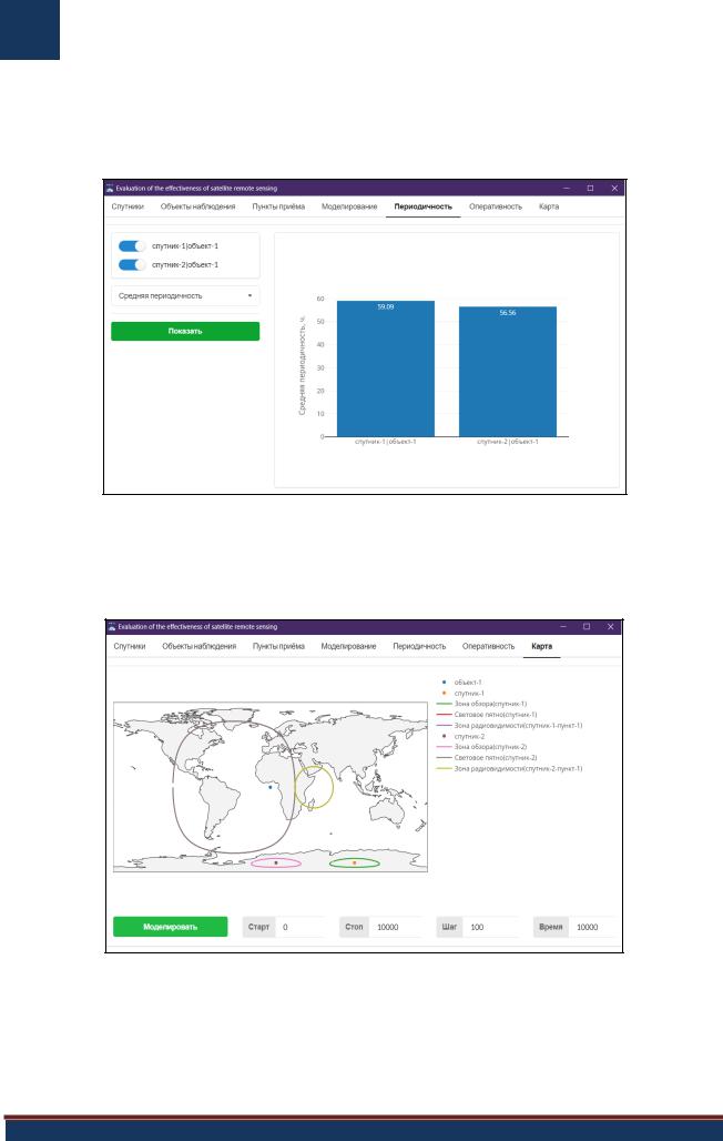
3.Для просмотра результатов моделирования существует две вкладки – «Периодичность» (рис. 3) и «Оперативность», они имеют схожий дизайн, слева расположены элементы управления: тумблеры включения результатов в итоговый график, под ними - выпадающий список с вариантами характеристик для отображения, ниже - кнопка построения графика, справа – графическая область.

Рис. 3. Результаты моделирования

4. Вкладка «Карта» (рис. 4) предназначена для графического моделирования, с целью подтверждения корректности вычислений, а также визуализации положения объектов системы в определённый момент времени.

Рис. 4. Графическое моделирование

В разработанном программном обеспечении было проведено имитационное моделирование для исследования зависимости показателя периодичности наблюдения КА от широты и от долготы объектов наблюдения. В первом случае (рис. 5) наблюдается явная тенденция к уменьшению показателя периодичности при увеличении широты, что доказывает непротиворечивость используемой модели. Во втором случае (рис. 6) зависимость тоже существует, но явных тенденций не наблюдается.

VII международная научно-практическая конференция | МЦНС «НАУКА И ПРОСВЕЩЕНИЕ»

<<< < Предыдущая 1 2 3 4 5 67 / 297 8 9 10 11 12 13 14 15 16 17 18 19 20 21 22 23 24 25 > Следующая >>>

Соседние файлы в папке книги2

#
24.02.20244.95 Mб0KON-465.pdf
#
24.02.202423.63 Mб2konf_15-24.pdf
#
24.02.2024627.85 Кб0M20_3222.pdf
#
24.02.2024331.75 Кб0mello_bozhja-ljubov.pdf
#
24.02.20246.97 Mб2Menedzhment_v_geologii_i_nedropolzovanii.pdf
#
24.02.20246.1 Mб1MK-1670.pdf
#
24.02.20243.31 Mб0MK-1907-2.pdf
#
24.02.20243.5 Mб0MNPK-566.pdf
#
24.02.20246.58 Mб1molodaya_nauka_2023_1.pdf
#
24.02.20243.82 Mб0MONOGRAFIYA_KM_EK_12_22-_el-set-izd_.pdf
#
24.02.20242.74 Mб0MONOGRAFIYA_KM_PP_11_21-_set_.pdf