

125 Кібербезпека / 4 Курс / 3.1_3.2_4.1_Захист інформації в інформаційно-комунікаційних системах / Лiтература / [Sumeet_Dua,_Xian_Du]_Data_Mining_and_Machine_Lear(BookZZ.org)
.pdf38 Data Mining and Machine Learning in Cybersecurity
The accuracy of random forest depends on the strength of the individual trees and a measure of the dependence between the trees. Moreover, the random forest algorithm uses bootstrap to avoid biases in tree building, such that cross validation (CV) is not needed in training and testing. However, random forest suffers from the class imbalance due to the maximization of the prediction accuracy in its algorithm. Tree-based methods have a high variance. The hierarchical structure of trees can produce an unstable result. The average of many trees, e.g., using bagging, can improve stability of ensemble learning algorithms.
2.1.2 Popular Unsupervised Machine-Learning Methods
2.1.2.1 k-Means Clustering
Clustering is the assignment of objects into groups (called clusters) so that objects from the same cluster are more similar to each other than objects from different clusters. The sameness of the objects is usually determined by the distance between the objects over multiple dimensions of the data set. Clustering is widely used in various domains like bioinformatics, text mining, pattern recognition, and image analysis. Clustering is an approach of unsupervised learning where examples are unlabeled, i.e., they are not pre-classified.
k-Means clustering partitions the given data points X into k clusters, in which each data point is more similar to its cluster centroid than to the other cluster centroids. The k-means clustering algorithm generally consists of the steps described as follows:
Step 1. Select the k initial cluster centroids, c1, c2, c3 …, ck.
Step 2. Assign each instance x in S to the cluster that has a centroid nearest to x. Step 3. Recompute each cluster’s centroid based on which elements are contained
in it.
Step 4. Repeat Steps 2 through 3 until convergence is achieved.
Two key issues are important for the successful implementation of the k-means method: the cluster number k for partitioning and the distance metric. Euclidean distance is the most employed metric in k-means clustering. Unless the cluster number k is known before clustering, no evaluation methods can guarantee the selected k is optimal. However, researchers have tried to use stability, accuracy, and other metrics to evaluate clustering performance.
2.1.2.2 Expectation Maximum
The expectation maximization (EM) method is designed to search for the maximum likelihood estimates of the parameters in a probabilistic model. The EM methods assume that parametric statistical models, such as the Gaussian mixture

Classical Machine-Learning Paradigms for Data Mining 39
model (GMM), can describe the distribution of a set of data points. For example, when the histogram of the data points is regarded as an estimate of the probability density function (PDF), the parameters of the function can be estimated by using the histogram.
Correspondingly, in EM, the expectation (E) step and the maximization (M) step are performed iteratively. The E step computes an expectation of the log likelihood with respect to the current estimate of the distribution for the latent variables, and M step computes the parameters that maximize the expected log likelihood found on the E step. These parameters are then used to determine the distribution of the latent variables in the next E step. The two steps are described as follows:
Step 1. (Expectation step) Given sample data x and undiscovered or missed data z, the expected log likelihood function of parameters θ can be estimated by θt:
f (θ |
|
θt ) = E[log L(θ; x, z)]. |
(2.23) |
|
Step 2. (Maximization step) Using the estimated parameter at step t, the maximum likelihood function of the parameters can be obtained through
θt +1 = arg max ( f (θ |
|
θt )). |
(2.24) |
|
|||
θ |
|
||
In the above, the maximum likelihood function is determined by the marginal probability distribution of the observed data L(θ; x). In the following, we formulate the EM mathematically and describe the iteration steps in depth.
Given a set of data points S = {x1,…, xm}, we describe the mixture of PDFs as follows:
K |
|
p(xi ) = ∑α j pj (xi ;θj). |
(2.25) |
j =1
In the above, αj is the proportion of the jth density in the mixture model, and
∑Kj =1
is the most employed, and has two parameters, mean μi and covariance Σj, such that θj = (μj, Σj). If we assume that θtj is the estimated value of parameters (μj, Σj) at the t-th step, then θtj+1 can be obtained iteratively. The EM algorithm framework follows:
m
αtj+1 = 1r ∑aijt , (2.26)
i =1
m
utj+1 = ∑i =1 aijt x j , (2.27) ∑mj =1 aijt
40 Data Mining and Machine Learning in Cybersecurity
|
|
m aijt (xi − utj )(xi − utj )T |
|||
∑tj+1 = ∑i =1 |
∑m aijt |
|
, |
||
|
|
|
i =1 |
|
|
aijt |
= |
ai p (x j ;uit , Σit ) |
|
. |
|
∑m ai p (x j ; uit , Σit |
) |
||||
|
|
i =1 |
|
|
|
(2.28)
(2.29)
These equations state that the estimated parameters of the density function are updated according to the weighted average of the data point values where the weights are the weights from the E step for this partition. The EM cycle starts at an initial setting of θ0j = (uj0, ∑0j ) and updates the parameters using Equations 2.26 through 2.29 iteratively. The EM algorithm converges until its estimated parameters cannot change.
The EM algorithm can result in a high degree of learning accuracy when given data sets have the same distribution as the assumption. Otherwise, the clustering accuracy is low because the model is biased.
2.1.2.3 k-Nearest Neighbor
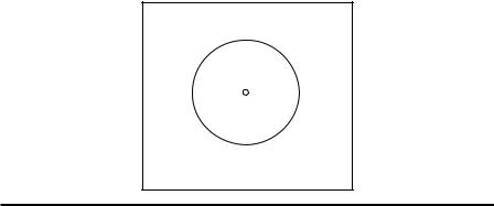
In KNN, each data point is assigned the label that has the highest confidence among the k data points nearest to the query point. As shown in Figure 2.8, k = 5, the
query point Xquery, is classified to the negative class with a confidence of 3/5, because there are three negative and two positive points inside the circle. The numbers of
nearest neighbors (k) and the distance measure are key components for the KNN algorithm. The selection of the number k should be based on a CV over a number of k settings. Generally, a larger number k reduces the effect of data noise on
–
––
+ |
– |
+ |
|
|
Xquery –
+
+
–
Figure 2.8 KNN classification (k = 5).
Classical Machine-Learning Paradigms for Data Mining 41
classification, while it may blur the distinction between classes. A good rule-of-thumb is that k should be less than the square root of the total number of training patterns. In two-class classification problems, k should be selected among odd numbers to avoid tied votes.
The most employed distance metric is Euclidean distance. Given two data
points in n dimensional feature space: x1 = (x11, …, x1n) and x2 = (x21, …, x2n ), the Euclidean distance between these points is given by
|
n |
|
0.5 |
|
|
∑ |
(x1i − x2i )2 |
|
|
dist (x1, x2 ) = |
|
. |
(2.30) |
|
i =1 |
|
|
|
|
Because KNN does not need to train parameters for learning while it remains powerful for classification, it is easy to implement and interpret. However, KNN classification is time consuming and storage intensive.
2.1.2.4 SOM ANN
SOM ANN, also known as Kohonen, characterizes ANN in visualizing low-dimen- sional views of high-dimensional data by preserving neighborhood properties of the input data. For example, a two-dimensional SOM consists of lattices. Each lattice corresponds to one neuron. Each lattice contains a vector of weights of the same dimension as the input vectors, and no neurons connect with each other. Each weight of a lattice corresponds to an element of the input vector. The objective of SOM ANN is to optimize the area of lattice to resemble the data for the class that the input vector belongs to. The SOM ANN algorithms consist of the following steps:
Step 1. Initialize neuron weights.
Step 2. Select a vector randomly from training data for the lattice.
Step 3. Find the neuron that has the weights most matching the input vector. Step 4. Find the neurons inside the neighborhood of the matched neurons in
Step 3
Step 5. Fine-tune the weight of each neighboring neuron obtained in Step 4 to increase the similarity of these neurons and the input vector
Step 6. Iteratively run Steps 1 through 5 until convergence
SOM ANN forms a semantic map where similar samples are mapped close together and dissimilar samples are mapped further apart. We can visualize the similarity by the Euclidean distance between weight vectors of neighboring cells. SOM preserves the topological relationships between input vectors.
2.1.2.5 Principal Components Analysis
The principal components analysis (PCA) represents the raw data in a lower dimensional feature space to convey the maximum useful information. The extracted
42 Data Mining and Machine Learning in Cybersecurity
principal feature components are located in the dimensions that represent the variability of the data. Given data set {x1, …, xn} in d-dimensional feature space, we put these data points in matrix X with each row presenting a data point and each col-
umn denoting a feature. We present the matrix X as X = [x1, …, xn]T, and transpose |
||
|
|
− |
as T. Then, we adjust the data points to be centered around zero by X − X , where |
||
− |
n×d |
, with each row presenting the mean of all rows |
X denotes the matrix in space ̂ |
|
|
in matrix X. Such an operation ensures that the PCA result will not be skewed due
to the difference between features. |
− |
|
Then, an empirical covariance matrix of X − X can be obtained by C = (1/d) |
||
− |
− |
− |
∑(X − X |
)(X − X )T. After we obtain the empirical covariance matrix of X − X , we |
|
then obtain a matrix V, V = [v1, …, vd], of eigenvectors in space ̂d, which consists of a set of d principal components in d dimensions. Each eigenvector vi, i = 1, …, m, in matrix V corresponds to an eigenvalue λi in the diagonal matrix D, where D = V −1CV and Dij = λi, if i = j; else Dij = 0. Finally, we rank eigenvalues and reorganize the corresponding eigenvectors such that we can find the significance of variance along the different orthogonal directions (denoted by eigenvectors). Then, we can present the ith principal component or eigenvector vi as follows:
vi = arg max |
|
|
|
((X − |
|
) − ∑(X − |
|
)v j vTj )v |
|
|
|
. |
(2.31) |
||
|
|
|
|
|
|
||||||||||
X |
X |
||||||||||||||
|
v |
=1 |
|
|
|
|
|
|
|
|
|
|
|
|
|
|
|
|
|
|
|
|
|
|
|
|
|
|
|
||
−
In the above equation, (X − X)vj captures the amount of variance projected along the direction of vj. This variance is also denoted by the corresponding eigenvalue λi. The application of the PCA method can be summarized in four steps as follows:
Step 1. Subtract the mean in each of the dimensions to produce a data set with a mean of zero.
Step 2. Calculate the covariance matrix.
Step 3. Calculate the eigenvectors and eigenvalues of the covariance matrix. Step 4. Rank the eigenvectors by eigenvalues from highest to lowest to get the
components in order of significance.
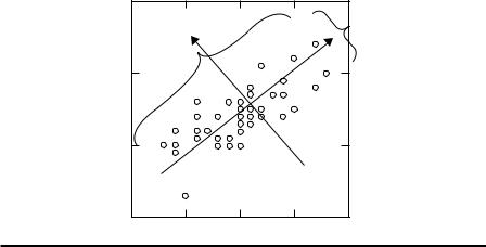
As shown in Figure 2.9, v1 and v2 are the first and second principal components obtained by PCA. λ1 and λ2 are the corresponding first and second eigenvalues. The principal components are orthogonal in feature space, while v1 represents the original variance in the data set and v2 represents the remaining variance.
PCA projects original data on a lower dimensional data space while retaining data variance as much as possible. PCA can extract uncorrelated features to describe the embedded statistical information of data sets. PCA has assumption that input data distribute continuously and normally, although non-normally distributed data may also result in good projection. However, when data spread in a complicated manifold, PCA can fail. PCA provides little visualization implications of the features in the original data sets.
Classical Machine-Learning Paradigms for Data Mining 43
4 |
|
|
|
|
|
v2 |
λ1 |
v1 |
λ2 |
3 |
|
|
|
|
2 |
|
|
|
|
1 |
3 |
5 |
7 |
9 |
|
Figure 2.9 Example of PCA application in a two-dimensional Gaussian mixture data set.
2.1.2.6 Subspace Clustering
In clustering methods, e.g., k-means, similar objects are grouped by measuring the distance between them. For high-dimensional data, objects are dispersed in space and distance, as the measure of “sameness” becomes meaningless (referred as the “curse of dimensionality”). Irrelevant dimensions act as noise, masking the clusters in a given data set. In order to reduce the number of dimensions, feature transformation (e.g., PCA in the next section) combines some attributes to produce a new attribute. However, since dimensions are not essentially eliminated, subspace clustering is not useful for clustering high-dimensional data with a number of irrelevant attributes. Feature selection is used to find the subset that contains the most relevant attributes. However, even this subset may have irrelevant attributes for some clusters. In addition, overlapping clusters will be ignored.
Subspace clustering, which performs a localization search and focuses on only a subset of dimensions, is an effective technique in such cases. This technique is similar to feature selection, except that instead of searching the entire data set, the subspace search is localized. The localization of the search makes it possible to find clusters from multiple and overlapping subspaces. The motivation for using subspace clustering is to remove the data that are not coherent with the clustered data. These data can be found by plotting data in the histogram charts with the dimensions as coordinate references.
Subspace clustering algorithms can be categorized as top-down or bottom-up. There are various bottom-up search methods like CLIQUE, MAFIA, cell-based clustering, CLTree, and density-based optimal projective clustering. All of the methods use the apriori style approach. In this style, if there are “n” units in “s”
44 Data Mining and Machine Learning in Cybersecurity
dimensions, then the s-dimensional data will be projected in (s − 1) dimensions. CLIQUE forms a cluster, and it discards the data in the cluster that are repeated during input. The cluster that is formed is represented using the disjunctive normal form (DNF). ENCLUS inherits all the characteristics of CLIQUE, except that it uses entropy to evaluate the clusters. MAFIA inherits all the characteristics of CLIQUE, and it introduces a new concept called parallelism. The cell-based clustering method fixes all the efficiency problems of the previous methods, and it uses an index structure to retrieve data from the clusters. The CLTree method evaluates by considering each cluster separately, unlike the previous methods. In the density-based method, the Monte Carlo algorithm is used to find the subset of data clusters that are not in coherence with other data in the cluster. In top-down subspace search methods, we have different types of methods such as PROCLUS, ORCLUS, FINDIT, and COSA. Readers should refer to L. Parsons, E. Haque, and H. Liu (2004) for details.
2.2 Improvements on Machine-Learning Methods
As discussed above, given a sample data set, a machine-learning algorithm can output a class label. The machine-learning methods have hypothesis that there exist unknown functions for a given sample data set. Using the given training data set, a family of hypotheses can be built, and then functions can be trained. A machinelearning model can be applied on the new data for classification or prediction. These classic machine-learning methods have common drawbacks when applied in cybersecurity applications. For example, classic machine-learning methods cannot use anomaly detection or other cyber defense analysis and decision procedures due to specific problems embedded in the cyber network data, e.g., imbalanced class distributions of normal and anomaly data.
2.2.1 New Machine-Learning Algorithms
Various new learning algorithms have been proposed to classify imbalanced data sets. The objective of these algorithms is to ensure the classification methods achieve optimal performance on unseen data. The representatives of the methods include one-class learners, ensemble methods, and cost-sensitive learners. Oneclass learners are trained to recognize samples from one class while rejecting samples from another class. In the training process, one-class data are used primarily to identify the minority class successfully. One-class learners are not stable, and the performance of one-class learners is strongly affected by the parameters and kernel used.
Cost-sensitive learners maximize a loss function associated with a databased cost matrix in which misclassification costs are different, e.g., the costs
Classical Machine-Learning Paradigms for Data Mining 45
|
+ |
True |
|
|
|
|
– |
|
|
+ |
TP |
|
FP |
|
|
|
|
||
Test |
|
|
|
|
FN |
|
TN |
|
|
– |
|
|
||
|
|
|
|
|
|
|
|
|
|
Figure 2.10 Confusion matrix for machine-learning performance evaluation.
for classification results in confusion matrix in Figure 2.10. In the confusion matrix, TP denotes true positive, TN denotes true negative, FP denotes false positive, and FN denotes false negative. The cost-sensitive methods improve the classification performance in imbalanced learning, although it is assumed that the cost matrix is available. Ensemble machine learning integrates the classification results of various classifiers into one classification result in a suitable fashion, such as by voting. This method attempts to generalize the task by training individual classifiers using randomly selected subsets of the data set. As long as each data subset is different, ensemble methods can provide a good discovery of the machine-learning task.
Two methods, bagging and boosting, resample the data set in ensemble classifiers. In the bagging ensemble, each classifier is trained using a different bootstrap of the data set. (Section 2.1.1.9 contains a detailed explanation of the bagging, boosting, and bootstrap methods.) The average bootstrap contains roughly 62% of the samples in the original data. Once each classifier is trained, the final classification result is determined by counting the majority of classifiers’ votes. Bagging performs well when individual classifiers can identify large differences in the classifications in the training data.
Boosting is used to weight the most difficult samples that are easily misclassified. In boosting, the probability of misclassification is increased, or vice versa for the series of classifiers. Ensemble methods can be valid only if there is disagreement among classifiers. A combination of classifiers cannot guarantee better performance than an individual classifier.
Additionally, researchers attempt to apply semi-supervised machine-learning methods to combat challenges in using labeled data sets for supervised learning, such as time consumption, expensiveness, limitation of expertise, and the accuracy of labels in collecting labeled data. Especially, semi-supervised learning has applications in cyber anomaly detection (Lakhina et al., 2004). Reinforced learning is a branch of machine learning, which considers the feedback from the finite states in an environment to adapt actions in the environment. Reinforced learning methods particularly have applications in multiagent environments in cyberinfrastructures. We recommend (Kaelbling et al., 1996; Chapelle et al., 2006) for more detailed analyses of semi-supervised learning.
46 Data Mining and Machine Learning in Cybersecurity
2.2.2 Resampling
As shown in Section 2.1.1.8, bootstrap, bagging, and AdaBoost are supervised machine-learning methods that use resampling. Similarly, other resampling methods are designed to improve classifier accuracies when used in conjunction with algorithms for training classifiers. For example, resampling is commonly used for imbalanced learning. Resampling adds samples to minority classes or reduces samples in majority classes in imbalanced data sets by using artificial mechanisms. The resampling data distribution is closer to a balanced data distribution.
Resampling methods can be classified into the following groups: random oversampling and undersampling, informed undersampling, and synthetic sampling with data generation. Undersampling is performed by reducing samples in the majority class. This technique may miss important information pertaining to the majority class. Oversampling replicates the minority samples, which causes overfitting. The synthetic sampling method generates synthetic data samples for the minority class by using clustering methods, such as finding the nearest neighbors to the current minority samples. This method may increase overlap between classes. Although none of these methods is perfect, studies have shown that sampling methods can improve the overall classification performance of classifiers over unbalanced data sets (H. He and E.A. Garcia, 2009).
2.2.3 Feature Selection Methods
Imbalanced data is commonly accompanied by high-dimensional feature space. Among the high-dimensional features, the existence of many noisy features can hinder and downgrade classifier performance. In the last few years, feature selection and subspace methods have been proposed and evaluated to solve this problem. Feature subset selection methods are used to select a small feature subset among highdimensional features according to feature selection metrics. It has been demonstrated that feature selection methods perform better than classification algorithms when imbalanced data have the characteristics of high-dimensional feature space.
Feature selection methods can be divided into two categories, feature scalar selection, which selects features individually, and feature vector selection, which selects features based on the mutual correlation between features. Feature scalar selection has the advantage of computation simplification and may not be effective for a data set with mutually correlated features. Feature vector selection methods select the best feature vector combinations.
Feature vector selection methods can be further divided into wrapper and filterbased methods. Wrappers use machine-learning methods, such as black box, and select the features that are most relevant, so that the learning method performs optimally. The search strategies include exhaustive search, beam search, branch and bound, genetic algorithms, greedy search methods, and so on. When wrappers are used, the selected features are prone to overfitting the data. In the filter-based

Classical Machine-Learning Paradigms for Data Mining 47
feature selection method, the feature is correlated with a class of features and its corresponding feature subset.
Using a correlation measure leads to an optimal solution in feature selection. Thus, the method focuses on two issues: the correlation measure criteria and the feature selection algorithm. The correlation criteria can be Pearson’s correlation coefficient (PCC), mutual information (MI), and other relevant criterions. PCC is a measure of linear dependency between variables and features. It is versatile to continuous or binary variables.
MI can measure nonlinear dependency, which measures the irrelevance of individual variables using the Kullback-leibler divergence. However, MI is harder than PCC to estimate, especially for continuous data. A typical filter-based feature selection method is sequential forward floating selection (SFFS), which finds the best approximation solution with regard to the number of selected features. SFFS starts from an empty feature selection pool and increases the pool using the local optimal feature set in two steps: inclusion and conditional exclusion steps. The heuristic basis of the SFFS algorithm is the assumption that the feature selection criteria are monotonic with the change of feature size and feature set information. SFFS approximates the optimal solution at an affordable computational cost.
2.2.4 Evaluation Methods
The traditional classification metrics include classification accuracy and error, defined as follows:
accuracy = |
# TP + # TN |
, |
(2.32) |
||
|
S |
|
|||
|
|
|
|
|
|
error = 1 − accuracy. |
|
(2.33) |
|||
The metrics are sensitive to the change in the data set and are effective when data are not balanced. For example, we have a data set that has a distribution in which 95% of samples are negative and 5% of samples are positive. If 5 of a given test data set of 100 samples are positive and 95 samples are negative, then, even if all test results are classified as negative, the accuracy is 95%. This value is preserved when the number of TN increases while the number of TP decreases the same amount. When the positive result is more important for researchers, the above metrics cannot provide the exact information of the class labels.
To comprehensively evaluate imbalanced learning, especially for minority classification, other metrics are used including precision, recall, F-score, Q-score, G-mean, receiver operating characteristics (ROC), areas under receiver operating characteristics, precision recall curves, and cost curves. The metrics are defined as follows:
Precision = |
# TP |
, |
(2.34) |
# TP + # FP |