

125 Кібербезпека / 4 Курс / 3.1_3.2_4.1_Захист інформації в інформаційно-комунікаційних системах / Лiтература / [Sumeet_Dua,_Xian_Du]_Data_Mining_and_Machine_Lear(BookZZ.org)
.pdf188 Data Mining and Machine Learning in Cybersecurity
Transversal endurance refers to the endurance of a proposed privacy preservation technique when it is applied in PPDM algorithms. A privacy preservation technique, such as a sanitization algorithm, is initially developed in pairs with a specific data-mining or machine-learning method. Given a number of data sets, the transversal endurance measures the ability of privacy protection provided by a variety of PPDM algorithms using the same privacy preservation methods.
Accompanied by the protection of sensitivity information, we need to consider the accuracy of mining results impacted by the loss of insensitive information. We call this metric functionality loss, because the modification of the original input data and new data-mining or machine-learning algorithms may lead to the downgrading data-mining or machine-learning results. Fundamentally, the functionality loss presents the difference between the mining results using the original data and the privacy preservation mining results using the modified data. Thus, this metric depends on both data set and PPDM algorithms. Various concepts have been proposed to present this metric in terms of data set, including accuracy, completeness, consistency, and so on.* Readers should refer to Bertina et al. (2005) for more details about these concepts. For example, the following classification error EC can present the total function loss of clustering algorithms:
K
EC = n1 ∑Clusterk ( X ) − Clusterk ( X M ), (8.2)
k =1
where |Clusterk(X)| and |Clusterk(XM)| denote the cardinalities of cluster k with the original data set X = {x1, …, xn} and modified data set XM = {xM1 , …, xMn }. With respect to association rules, function loss refers to the loss of nonsensitive rules. This loss results from the application of privacy preservation techniques that hides both sensitive and insensitive information.
Computation complexity evaluates the time requirements of privacy preservation algorithms. The proposed approaches include calculating the CPU time used by the algorithm measuring the operations needed for hiding the sensitive information and measuring computational cost by the degree of a polynomial. In SMC, we must include the communication cost in the final computation cost, which is caused by the amount of exchanged information between sites.
Scalability evaluates the efficiency of PPDM algorithms with the increasing amount of input data. The proliferation of information communicative techniques and data storage capabilities requires the development of more efficient PPDM algorithms to deal with the influx of data sets. Moreover, the increasing data dimensionality exacerbates the design of high-scalable PPDM methods.
*Completeness measures the loss of individual data information in the sanitized data; consistency measures the loss of correlation between data in the sanitized data.
Privacy-Preserving Data Mining 189
8.3Data-Mining and Machine-Learning Applications in PPDM
The objective of PPDM is to keep private data and private knowledge safe once the mining on the data has been completed. PPDM methods can be analyzed from the perspectives of data distribution, data modification, data mining algorithms, data or rule hiding, or privacy preservation (Verykios et al., 2004a). We categorize the principle PPDM methods in Table 1.1, according to data-mining algorithms and present their privacy preservation methods. In particular, the privacy preservation technique is the most important for the selective modification of the data, which are classified into three groups: heuristic-based techniques, cryptography-based techniques, and reconstruction-based techniques. For a more detailed analysis, readers should see Verykios et al. (2004a).
Researchers have investigated various data-mining algorithms in isolation of each other. Among them, the most important privacy preservation methods have been proposed for a number of data-mining algorithms, like support vector machines (SVM) classification (Yu et al., 2006), association rule mining algorithms (Evfimievski et al., 2004), K-means clustering (Vaidya and Clifton, 2003), decision tree inducers (Agrawal and Srikant, 2000), BN (Wright and Yang, 2004), KNN (Kantarcioglu and Clifton, 2004), ANN (Barni et al., 2006), and other statistical methods (Du et al., 2004). Readers should see Table 1.1 for our list of references on this topic.
8.3.1 Privacy Preservation Association Rules (Table 1.1, A.4)
Let us review the association rules as explained in Chapter 2. Let E = {I1,I2, …, Ik} be a set of items and X be a database consisting of n transactions T1, …, Tn, X = {T1, …, Tn}. Each transaction Tj, 1 ≤ j ≤ n is a subset of items with Tj ̂ E. Each transaction Tj has support s (Ti) in E, defined by the following conditional probability:
s (Ti ) = |
#(t X |Ti t ) |
. |
(8.3) |
|
|||
|
n |
|
|
Given a threshold Th, if s (Tj) ≥ Th, we say transaction Tj is frequent; if we have another transaction Ti ̂ E and Tj ̂ Ti, we say s (Tj) ≥ s (Ti).
Itemset I causes a privacy breach of level ρ, if we randomize transaction Tj = R(Tj ), and we find that a frequent itemset I and the item Ir I have the conditional probability
P (Ir Tj |
|
I Tj ) ≥ ρ. |
(8.4) |
|
190 Data Mining and Machine Learning in Cybersecurity
To solve this problem, Evifimievski et al. proposed randomization operators using “cut and paste” to insert “false” items to replace some true items (Evfimievski et al., 2002). Their method includes three steps as follows:
Step 1. Randomly select an integer number N between 0 and the cutoff Km. Step 2. Randomly select N items in transaction Tj and put them in the empty
transaction Tj .
Step 3. Select items in the remaining set E = {I1 , I2 , …, Ik } with probability ρm and continue to fill them in Tj .
In the above, transaction Tj has size m, and two parameters Km and ρm are optimized based on the desired level of privacy.
Using the notations as defined above, itemset I and X = {T1, …, Tn} were defined as |I| = d and |Ti| = m, i = 1, …, n. Then, using the definition of support given in Equation 8.3, the authors obtained partial support for itemset I as follows: ̂s =
(s0, …, sd) and sl = #{Tj X|#(I ∩ Tj) = l }/n.
They proposed a transition matrix M, to transform the original support of itemset I, ̂s , to the randomized support of its subsets, ̂s ′. Matrix M has d rows and m columns, and the following definition for each element at row l ′ and column l:
Ml l = P |
# (Tj ∩ I )= l | (Tj ∩ I ) = l . |
(8.5) |
|
|
|
The transformation between ̂s |
and ̂s ′ is as follows: |
|
|
E(s ) = M s , |
(8.6) |
where E(̂s ′) denotes the expected value of the randomized partial support vector ̂s ′ and ̂s ′ follows multinomial distribution. Using Equation 8.6, the original partial support vector can obtain its unbiased estimator as
|
|
(8.7) |
suest = M −1 |
s , |
and the variance matrix for this estimator as
d
Cov(suest ) = n1 ∑sl P −1 D [l ](P −1 )T , (8.8)
l =1
where matrix D[l] has k + 1 rows and k + 1 columns, and each element D [l ]iD , jD =
PiD ,l δiD = jD − PiD ,l PjD ,l , iD = 1, ..., d , jD = 1, ..., m .

Privacy-Preserving Data Mining 191
Using the above randomization and randomized support analysis, the privacy preservation apriori association rules can be mined in the following steps:
Step 1. Initialize k = 1.
Step 2. Randomize the original data, and estimate partial support and variance σ2 of each candidate set using Equations 8.7 and 8.8.
Step 3. Keep those candidate sets that contain support values above the minimum support threshold smin.
Step 4. Form new candidate sets with all (k + 1)-sized itemsets that have k-sized sub-itemsets with all support values above smin − σ.
Step 5. Return to Step 2 with k = k + 1 and repeat steps until no candidate remains or the estimator deviates from the expected value significantly.
As shown in Figure 8.6, Evifimievski et al. proposed a framework for privacy preservation association rules mining from transactions by randomization methods. They evaluated the privacy breach level by checking Equation 8.1 and obtained the conditional probability by
P (Ir Tj |
|
I |
T j )= |
∑d |
sl+ Pdl |
(8.9) |
|
|
l =0 |
, |
|||||
|
|
|
|
|
|
|
|
|
|
|
|
∑d |
sl Pdl |
|
|
|
|
|
|
|
|||
|
|
|
|
l =0 |
|
|
|
where sl+ = P (#(Tj ∩ I )= l , Ir T j ), s0+ = 0 .
Collection of original data
Randomization of the original data
PP association rules mining
Evaluation of privacy breach
Figure 8.6 Workflow of privacy preservation association rules mining method. (Reprinted from Inform. Syst., 29, Privacy preserving mining of association rules, Evfimievski, A., Srikant, R., Agrawal, R., and Gehrke, J., 343–364, Copyright (2004), with permission from Elsevier.)
192 Data Mining and Machine Learning in Cybersecurity
They defined the lowest discoverable support (LDS) as the support of an itemset 4σ away from zero. Then, mutual interaction between LDS and the privacy breach level can demonstrate the relation between rules discoverability and privacy breach level. They used two real data sets in the experiments. The first (soccer) data set consists of the click stream log from the 1998 World Cup Web site. Each transaction denotes a session of a user’s access to the Web site, and each item denotes an HTML request. The soccer data set includes 11,000 HTMLs and 6,525,879 soccer transactions. The mail order data set consists of order transactions from an online market. Each transaction denotes a sequence of items purchased by a single order. The mail order data set includes 96 items and 2,900,000 transactions.
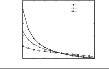
As shown in Figure 8.7, where one transaction has five items, the LDS decreases when the privacy breach level increases by a great deal. This figure demonstrates that a higher breach level needs a much lower LDS for 3-itemsets. A higher breach level indicates a weaker randomization level or a lower hidden ability. A 3-itemset has a lower LDS than 1-itemset at higher privacy breach levels, e.g., from 65% to 90%. This phenomenon occurred because of the large number of false items involved in the randomization process. Because the 3-itemset involved fewer false positives than the 1-itemset at a higher breach level, discovering the 3-itemset became easier than discovering the 1-itemset.
Lowest discoverable support, %
2.5 |
|
|
|
|
|
|
|
|
|
|
|
|
|
3-itemsets |
|
|
|
|
|
|
|
2-itemsets |
|
2 |
|
|
|
|
|
1-items |
|
1.5 |
|
|
|
|
|
|
|
1 |
|
|
|
|
|
|
|
0.5 |
|
|
|
|
|
|
|
0 |
|
|
|
|
|
|
|
30 |
40 |
50 |
60 |
70 |
|
80 |
90 |
|
|
|
Privacy breach level, % |
|
|
||
Figure 8.7 LDS and privacy breach level for the soccer data set. (Reprinted from Inform. Syst., 29, Privacy preserving mining of association rules, Evfimievski, A., Srikant, R., Agrawal, R., and Gehrke, J., 343–364, Copyright (2004), with permission from Elsevier.)
Privacy-Preserving Data Mining 193
Evifimievski et al. experimented on both data sets by choosing a privacy breach level of 50% and a minimum support threshold of LDS. They reported high coverage of the predicted rules, a high true positive, and low false positive rates.
8.3.2 Privacy Preservation Decision Tree (Table 1.1, A.6)
Given a data set partitioned into two parts, Du and Zhan attempted to solve the MPC problems using a decision-tree classifier (DTC) (Du and Zhan, 2002). They built a protocol that allows two partners to classify the data set without compromising either’s privacy.
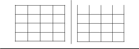
Du and Zhan partitioned the data set into two feature sets: {f1,…,fk} and {fk,…, fd}, and grouped the data composed by the feature set { f1, …, fk} into group A and the data composed by the feature set { fk+1, …, fd} into group B (see Figure 8.8). They denoted these two groups of data as SA and SB, respectively.
As noted in Section 3.3.5.1, decision-tree classification consists of two procedures: tree building and tree pruning. In the tree-building procedure, the splitting of nodes depends on the splitting criteria. The best split can equal the discovery of the largest information gain among features. To calculate entropy, Du and Zhan first estimated the probability of class j in sample data as follows:
|
|
ˆ |
|
|
Pj = |
Pj |
, |
||
|
S |
|
||
|
|
|||
|
|
|
|
|
where
ˆ
Pj denotes the number of class j in data set S |S| denotes the cardinality of data set S
ˆ
They obtained Pj using the following equations:
Pˆj = VA (VB Vj ) or Pˆj = (VA Vj ) VB ,
(8.10)
(8.11)
where VA, VB, and Vj denote feature vectors of size d, respectively for SA, SB and the data in S belonging to the jth class. If data point Si in group A (B) (see Figure 8.8)
Group A
f1 |
. . . |
fk |
S1
. . .
Sn
|
Group B |
|
|
|
|
fk |
. . . |
fd |
|
S1
. . .
Sn
Figure 8.8 Partitioned data sets by feature subsets.
194 Data Mining and Machine Learning in Cybersecurity
satisfies the requirement that only considers group A’s (B’s) feature set, the vector VA(VB) = 1; otherwise, VA(VB) = 0. If data point Si belongs to class j, then vector Vj(i) = 1; otherwise Vj(i) = 0. Using equations in Section 3.3.5.1, information gain can be calculated.
Using the above DTC, a data point (A1, …, Ak, Bk+1, …, Bd), where (A1, …, Ak) and (Bk+1, …, Bd) denote the known part in group A and known part in group B
respectively, can be classified as follows. Group A (B) traverses the tree separately. In the tree traverse by group A (B), for any node split by the feature in group A (B), its respective child will be traversed according to the data value; for any node split by feature in group B (A), all children of the node are traversed by group A (B). All the leaf nodes that are reached by group A (B) are recorded in a respective vector
TA (TB).
Since finding a trusted third party to combine the groups is unfeasible, Du and Zhan solved the problem using the commodity server (CS) model. In this model, the third party is not allowed to participate in computation, not allowed to gain knowledge of private data and computation result from A and B, and not allow to collude with both sides. Based on these assumptions, they computed the scalar product of the private data sets belonging to group A and B, respectively. Given private vector VA from group A and private vector VB from group B, the scalar product was calculated between VA and VB as follows:
VA VB = ∑VA (i) VB (i). |
(8.12) |
The scalar product protocol using CS consists of the following steps:
Step 1. CS generate random vectors VRA and VRB and random numbers rA and rB for group A and group B, respectively, where VRA VRB = rA + rB.
Step 2. Group A (B) sends VA = VA +VRA (VA = VB +VRB) to group B(A). Step 3. Group B sends VAVB + rB to group A.
Step 4. Group A derives VA · VB from (VA VB + rB ) −VRA VB + rA.
The proposed framework is efficient, but the assumption that the third party should not collude with either source poses challenges for implementation. The proposed algorithm may cause an information breach in two ways: the scalar product results or design of the privacy preservation framework. They also did not test the proposed scheme in real and complex data sets.
8.3.3 Privacy Preservation Bayesian Network (Table 1.1, A.2)
Using the vertically partitioned data of two groups SA and SB, in Section 8.3.2, we discuss the technique of privacy preservation Bayesian networks (PPBN). In PPBN, the objective is to learn Bayesian network (BN) structure on the combination of
Privacy-Preserving Data Mining 195
data sets SA, held by Alice, and SB, held by Bob, and prevent privacy leaks between Alice and Bob. Each participant, Alice or Bob, only receives knowledge of the BN structure but no confidential information from the other partner.
Yang and Wright (2006) presented a protocol to construct a BN for vertically partitioned data. We use the notations and definitions presented in the Section 3.3.6.1 BN classifier to simplify the description of PPBN. Two research topics exist in the BN classifier: the recognition of BN structure and the training of BN model. Wright and Yang employed the K2 algorithm (Yang and Wright, 2006) in learning the BN structure and modified the scoring function in the K2 algorithm. Given a set of v variables or nodes, X = {x1, …, xi, …, xv}, the K2 algorithm attempts to maximize the score function f(xi,parent(xi)) in the sequence of parent candidates (nodes) up to a maximum of u (the number of upper bound) parents for a node. K2 consists of the following steps.
Step 1. Initialize parent set parent (xi) to be empty for each node, i = 1, …, v.
Step 2. Update f (xi, parent (xi)) with f (xi, parent(xi)) (cparent(xi) − parent(xi)), if f (xi, parent(xi)) < f (xi, parent(xi)) (cparent(xi) − parent(xi)); otherwise stop adding parents to node xi, where cparent(xi) refers to the pool of possible parents of node xi and parent(xi) refers to the pool including the selected parent nodes.
Step 3. Iterate Steps 1–2 until node xi has obtained u parents.
Step 4. Iterate Steps 1–3 until all nodes in the BN have been added as parents.
In the original K2 algorithm, the score function has the following definition for binary attributes:
qi |
Pij 0 ! Pij1 ! |
|
|
|
f (xi , parent(xi )) = ∏ |
, |
(8.13) |
||
(Pij 0 + Pij1 +1)! |
||||
j =1 |
|
|
||
|
|
|
where qi denotes the number of unique parents of variable xi, Pijk,k = 0 or 1 denotes the number of occurrences of variable xi taking value k and its parent(xi) taking the jth unique value. To preserve privacies in BN computation, Wright and Yang proposed a new score function as follows:
qi
g(xi , parent(xi )) = ∑12 (ln Pij 0 + ln Pij1 − ln(Pij 0 + Pij1 + 1))
j =1
+ (Pij 0 ln Pij 0 + Pij1 ln Pij1 − (Pij 0 + Pij1 + 1)ln(Pij 0 + Pij1 + 1)).
(8.14)
196 Data Mining and Machine Learning in Cybersecurity
Yang and Wright obtained this score function via the operation of a natural log on the score function in Equation 8.13 and simplified processing with respect to Stirling’s approximation. The log function and approximation have no effects on the ordering of the parent nodes in the K1 algorithm, while the operations preserve the original score information in the new score function. Following the example above, we will use Alice and Bob to illustrate the authors’ point. In the implementation of the g score function in the K2 algorithm, Alice and Bob jointly solved the maximum g scores associated with the parent nodes. In the proposed PPNB method, privacy-preserving protocols were employed on scalar products, computations of Pijk, score computations, and score comparisons. Alice and Bob shared the intermediate values of the above four computation results.
Wright and Yang designed a privacy-preserving scalar product protocol as follows. Given private vector VA from Alice and VB from Bob, the proposed scalar product protocol consisted of the following steps:
Step 1. Alice generated an encryption key and a decryption key using an encryption algorithm, and shared the encryption with Bob.
Step 2. Alice encrypted her private data elements in VA, E(VA1), …, E(VAn), and shared the encrypted data with Bob.
Step 3. Bob encrypted a random number R, obtained the encrypted R, E(R), and shared the encrypted data E(R) ∏yi with Alice, where if VAi = 1, yi =
E(VAi); otherwise yi = 1.
Step 4. Alice derived R + VA · VB from E(R) ∏yi .
In the above, Wright and Yang demonstrated that E(R) ∏yi = E(VA VB + R) in
Step 3, such that Alice could obtain R + VA · VB using the description key while Bob only maintained R. With respect to the computations of privacy-preserving parameters Pijk, both Alice and Bob generated a respective n-length vector compatible with i, j, k. Then, both partners obtained the shared parameters Pijk via the above private scalar product protocol. The output was the random shares of parameters Pijk.
In private score computation, Wright and Yang referred to Yang and Wright
(2006) for computing random shares of ln Pijk and Pijk ln Pijk. With respect to (Pij0 + Pij1 + 1) ln (Pij0 + Pij1 + 1), they let Alice and Bob separately compute
random shares. Then, Alice and Bob selected the maximum values among the m shared score values. Yang and Wright (2006) evaluated the proposed g score function on two data sets. The first (Asia) data set included eight features such as Asia, smoking, tuberculosis, lung cancer, bronchitis, either, x-ray, and dyspnoea. The second (synthetic) data set consisted of 10,000 data points and six features denoted 0–5. Wright and Yang compared the performance of the g and f score functions in both data sets and observed that the g score function approximated the f score function sufficiently for the K2 algorithm, e.g., all g scores fall into 99.8% of ln(f ). They noted several causes of information leaks: known structure
Privacy-Preserving Data Mining 197
of BN, sequence of edges included in BN, and parameters of BN model, which were associated with particular features.
8.3.4 Privacy Preservation KNN (Table 1.1, A.7)
As explained in Section 2.3.2.3, KNN classifies a query data point xquery into the majority class of its neighborhood. This neighborhood is defined by a distance
function d(xi, xquery) and the k nearest neighbors measured by the distance to the query data point. In an SMC problem, the entire data set {xj}, j = 1, …, n, is
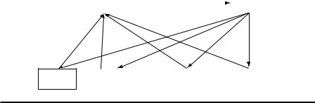
composed of multiple data sets located at different sites site 1, …, site N. As shown in Figure 8.9, each site i, where i = 1, …, N, holds a part of the horizontally partitioned data Si. Hence, the whole data set can be expressed as S = i Si . Without considering the privacy-preserving issues, the k closest neighbors can be found in S for the query data point x and the majority class among the k neighbors labels data point x. In privacy preservation KNN calculation, each site prevents its private data from leaking to the other sites while serve as a participant in obtaining the k nearest neighbors for the query data.
Kantarcioglu and Clifton (2004) presented a framework using a privacy-pre- serving KNN method to mine horizontally partitioned databases. Hence, the feature space remained the same among all participants. They assumed each set of databases is able to conduct KNN separately. They attempted to find the local KNN results most similar to the global KNN results, and to obtain most of the global KNN results. The third party, C and O in Figure 8.9, is a not trusted but is a non-colluding party.
In the proposed privacy preservation KNN method, Kantarcioglu and Clifton first obtained N*k local nearest neighbors among all of the N partners in an untrusted site C. Second, they combined the local KNN results, and obtained the final global classification result, which they then sent to site O. The private information considered in the procedures included original location of the local nearest neighbors and their distance values, and the global class labels assigned to the data points.
Site C |
|
|
Site O |
|
|
||
|
|
|
|
Site 1 |
|
|
Site 2 |
Site i |
|
|
Site N |
||
S1 |
|
|
|
S2 |
, . . . , |
Si |
, . . . , |
SN |
|
|
|
|
|
|
|
|
|
||
Figure 8.9 Framework of privacy preservation KNN.