125 Кібербезпека / 4 Курс / 3.1_3.2_4.1_Захист інформації в інформаційно-комунікаційних системах / Лiтература / [Sumeet_Dua,_Xian_Du]_Data_Mining_and_Machine_Lear(BookZZ.org)

148    Data Mining and Machine Learning in Cybersecurity

Here, TP refers to the conditional probability describing the cases in which the connection is really launched by scanners and the sequential hypothesis is correct. FP refers to the conditional probability, which denotes the cases in which benign users launch the connection but the hypothesis is that scanners launched the connection. We prefer to specify thresholds α and β to both TP and FP, such that

Given observation S = {S1, …, Sn} including n connection attempts, the likelihood ratio is calculated as follows:

n

Λ(S) = ∏ Pi1 , (6.4)

i =1 Pi0

where Pi1 denotes the discrete probability distribution of connection to host Si when the hypothesis is that a scanner launched the connection, and Pi0 is the corresponding conditional probability distribution when hypothesis is benign. This ratio was assigned an upper bound η1 and lower bound η0 to accept the hypotheses that a given remote source is either a scanner or benign. They were expressed as η0 ≤ Λ(Y ) ≤ η1. Using statistical test equations in Equation 6.3, Jung et al. deduced the approximate solutions to these two bounds as

Readers can refer to Jung et al. (2004) for more information regarding the deduction process.

Using the above bounds solution, the real-time scan detection algorithm consists of the following steps:

Step 1. Collect sample data and update sample data set S. Step 2. Calculate Λ(S) using Equation 6.4.

Step 3. If Λ(S) ≥ η1, classify the observed event S as a scanner; if Λ(S) ≤ η0, classify the observed event S as benign. Otherwise, return to Step 1.

In the above steps, a detect decision corresponds to a random walk with regard to the two thresholds. In Step 1, only the sample data that has a new destination will be added to update the sample data set.

Using an analysis of traces from two qualitatively different sites, it is shown that TRW requires a much smaller number of connection attempts (four or five) to detect malicious activity than previous schemes, while also providing theoretical bounds on the low (and configurable) probabilities of missed detections and false alarms.

Machine Learning for Scan Detection    149

Table 6.1 Testing Data Set Information

Source: Jung, J., Paxson,V., Berger, A.W. and Balakrishnan, H., Fast portscan detection using sequential hypothesis testing, in IEEE Symposium on Security and Privacy, Oakland, CA, © 2004 IEEE.

The authors conducted experiments on two groups of network traffic data sets, collected by the Lawrence Berkeley National Laboratory (LBL) and the International Computer Science Institute (ICSI) at the University of California, Berkeley. The LBL data set is sparser than the ICSI data set (as shown in Table 6.1). Both data sets had entries of TCP connection logs labeled as “successful,” “rejected,” and “unanswered.” The remaining entries were of undetected scanners. The TP and FP rates obtained from TRW were compared with those obtained from SNORT and BRO. The authors selected α = 0.99 and β = 0.01 in the experiments. TRW showed the highest TP detection rate, while maintaining a lower FPR. In this experiment, the significant advantage of TRW was speed. It required only four or five connection attempts to detect scans. However, attackers sometimes used this method to deny the legitimate source connectivity by deceiving scanning behavior.

Application Study 4: Using Expert Knowledge-Rule-Based Data-Mining Method in Scan Detection (Table 1.5, E.4)

Simon et al. (2006) formulated scan detection as a data-mining problem. They attempted to apply data-mining approaches to build machine-learning classifiers based on the labeled training data set and proportional feature selection. Then, they employed the learned machine-learning model to detect scanners.

Given a set of network traffic traces, they extracted each trace as a pair of source IP and destination port, SIDP or <source IP, destination Port>. They classified normal users and scan attackers who used the same destination ports but accessed them from

150    Data Mining and Machine Learning in Cybersecurity

SIDPs

Feature extraction

Rule-learning classifier

Report scanners

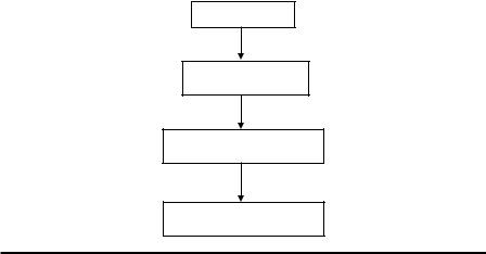
Figure 6.5 Workflow of scan detection using data mining in Simon et al. (2006). (From Simon, G. et al., Scan detection: A data mining approach, in: Proceedings of the Sixth SIAM International Conference on Data Mining (SDM), Bethesda, MD, pp. 118–129, 2006. With permission.)

different source IPs. As shown in Figure 6.5, the designed scan detection method followed the workflow of traditional data-mining methods. In feature extraction, they introduced four sets of features to integrate expert knowledge. Among these feature sets, three sets were useful for the classification of SIDPs.

The first set included four statistical features of a destination IP and port, e.g., the averaged number of distinct destination IPs over all destination ports that source IP had attempted to connect. The second set included six statistical features of source IPs, which described the role and behaviors of the source IPs, e.g., the ratio of distinct destination IPs that attempted to connect by the source IP that did not provide any service on destination ports to any source. The third set included four statistical features of individual destination ports, e.g., the ratio of a distinct destination IP that attempted to connect by the source IP that did not provide any service on destination ports to any source. Readers should refer to Simon et al. (2006) to learn the definition of features in the three extracted feature sets of the network traces.

Simon et al. (2006) selected a rule-based learning classification algorithm, RIPPER (proposed by Cohen [1995]), as their classifier because of the efficiency and effectiveness of RIPPER in dealing with imbalanced and nonlinear data. RIPPER elicits classification results in the form of rules.

In their experiments, Simon et al. collected network traffic traces for 2 days from an infrastructure at the University of Minnesota consisting of five networks and a number of subnetworks. They constructed one sample set every 3 h and finally obtained 13 sample sets. They used the first sample set as a training set and

Machine Learning for Scan Detection    151

the other 12 sample sets as testing sets. The length of observation adapted to the sufficient and necessary classification of SIDPs. Simon et al. labeled all SIDPs in five groups: scan, p2p, noise, normal, and unknown. They evaluated the proposed data-mining method by measures: precision, recall, and F-score (see their definition in Chapter 1). The scan detection results were compared to those obtained using TRW. The authors selected multiple thresholds to find the most competitive performance of TRW.

The experimental results showed that the proposed method outperformed TRW in all three measures. The proposed method also showed consistent performance among all 12 testing data sets. The F-score was maintained above 90% corresponding to a high precision rate and a low FPR. They attributed the success of the proposed method to its ability to correlate one source IP address with multiple destination IP addresses. The correlation allowed the rule-based learning method to detect scanners earlier. In addition, they found that the proposed method could detect scans in a short time, based on the trained model using training data obtained over a long time. In experiments, Simon et al. tested the collected data set that was collected in 3 days, in a 20 min time window.

These experiments showed that data-mining models can integrate expert knowledge in rules to create an adaptable algorithm that could substantially outperform the state-of-the-art methods, such as TRW, for scan detection in both coverage and precision.

Application Study 5: Using Logistic Regression in Horizontal and Vertical Scan Detection on Large Networks

Gates et al. (2006) developed logistic regression modeling for scan detection in large cyberinfrastructures that have the following characteristics: huge volume flow-level traffic data, multiple routers for data collection, multiple geographic and administrative domains, and unidirectional traffic flow.

Given a set of network traffic traces, Gates et al. extracted events from the traffic traces of each single source IP, which were bounded by quiescent periods. They sorted the traffic traces in each event according to destination IP and ports. They extracted 21 statistical features for scan detection, e.g., ratio of unique source ports to number of traffic traces. Based on the statistical analysis of the contribution of each feature to the scan detection, they selected the most significant six features for each event. These six features include the percentage of traces that appear to have a payload, the percentage of flows with fewer than three packets, the ratio of flag combinations with an ACK flag set to all flows, the average number of source ports per destination IP address, the ratio of the number of unique destination IP addresses to the number of traces, and the ratio of traces with a backscatter-related flag combination such as SYN-ACK to all traces. They used these six features as input in logistic regression model to calculate the probability of an event containing a scan,

152    Data Mining and Machine Learning in Cybersecurity

In the above equation, fi denotes the selected features for logistic regression calculation, and n = 6. α0, …, αn are coefficients determined by both experts and the training data set.

In the experiment, Gates et al. split data sets into three groups: elicitation, training, and testing. They collected elicitation traffic traces, which included 129,191 events, for 1 h (Muelder et al., 2007). They collected training traffic trace sets in the subsequent hour and included 130,062 events. Then, they collected 127,873 testing events in the following hour after collecting and training the data set. They randomly selected three groups of data with respect to the three data sets: elicitation, training, and testing. These three groups consisted of 100, 200, and 300 sample data, respectively.

The expert manually labeled each of the events as containing a scan or not containing a scan. The same expert was involved in labeling events as scanned or not scanned. The elicitation group included 30 randomly selected observations and the 70 observations with the largest variances. Using the values of the 21 features, the expert estimated the probability of an event containing a scan. They used the estimated probabilities to determine the coefficients’ prior values in Equation 6.6. Combined with the training data set, they estimated the posterior feature coefficients using the Bayesian approach. Furthermore, they selected the six most significant features and their corresponding coefficients in the regression model using the Akaike Information Criterion (AIC).*

Then, they input the 300 testing data into the learned regression model to generate an estimated probability for each event. If the probability was greater than 0.5, the event was classified as a containing scan; otherwise, it was classified as normal. Using the ground truth labeled by the expert, the authors obtained the detection rate and FAR at 95.5% and 0.4%, correspondingly. They also conducted performance compassion between the proposed method and TRW (α = 0.01 and β = 0.99) on the same training and testing data set, and found that the proposed method obtained as high detection accuracy as the TRW did. However, this proposed scan detection method cannot be implemented in real-time applications

*AIK measures the fitness of a regression model for a given data set. AIK is mostly employed for model selection. Generally, the selected model corresponds to the lowest AIC for the given data set. The commonly used equation for calculating AIC is AIC = 2k − 2 ln(L), where k denotes the number of coefficients in the regression model and L denotes the maximized likelihood of the estimated model.

Machine Learning for Scan Detection    153

due to its requirement of the collection of sufficient flow-level traffic flows for a single source IP.

Application Study 6: Using Bidirectional Associative Memory and ScanVis in Scan Detection and Characterization (Table 1.5, E.5)

Muelder et al. (2007) presented a study on how to use associative memory-learning techniques to compare network scans and create a classification that can be used by itself or in conjunction with visualization techniques to better characterize the sources of these scans. These scans produced an integrated system of visual and intelligent analysis, which is applicable to real-world data.

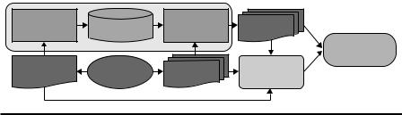
As shown in Figure 6.6, the proposed method consists of four steps in scan detection and characterization: the collection and labeling of network traffic data, the training of bidirectional associative memory (BAM) using the controlled scan data, the classification of network unknown traffic scan data using the learned BAM model, and the visualization and characterization of scan patterns. Controlled scan data are the set of scan data of which we know the properties, such as the source IP and ports, source hardwire and software, and so on.

The first three steps focus on scan classification, as with the other supervised machine-learning methodologies that we have discussed in the previous sections. The fourth step is an additional contribution to the in-depth analysis of scan patterns that enables cyber administrators to perform respective controls over the detected scans. Muelder et al. (2007) assumed scan detection was performed using the existing data-mining techniques, and controlled data were available for classification. Thus, the focus of the research was in the BAM classification process, and the application of ScanVis (Muelder et al., 2005) was in scan characterization.

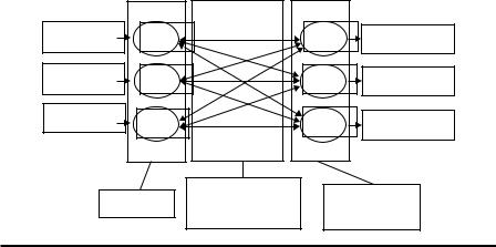
BAM maps from one pattern space, e.g., layer X, to another pattern space, e.g., layer Y, by using a two-layer associative memory, as shown in Figure 6.7.

Figure 6.6 Workflow of scan characterization in Muelder et al. (2007). (With kind permission from Springer Science+Business Media: Proceedings of the Workshop on Visualization for Computer Security, Sacramento, CA, Intelligent classification and visualization of network scans, 2007, Muelder, C., Chen, L., Thomason, R., Ma, K.L., and Bartoletti, T., Copyright 2007.)

154    Data Mining and Machine Learning in Cybersecurity

Figure 6.7 Structure of BAM.

The associative memory consists of a weight matrix wij , and the weight wij corre-

m*n

spondstothemappingfrominputneuronxi toyj withwij = ∑Pp=1 Input p,i Output p, j ,

where p is the index of patterns, i = 1, …, m and j = 1, …, n. Given detected scans and their corresponding patterns, we can generate the weight matrix as a classifier for the scans in the similar patterns. The mapping between the pair xi and yj

can be performed as follows: if Inputpi · wij > 0 (wij · Outputpj > 0), Output(p+1)i = 1 (Input(p+1)i = 1), Inputpi · wij < 0 (Outputpj · wij < 0) Output(p+1)i = −1 (Input(p+1)i = 1), or

Output(p+1)i = Outputpi (Output(p+1)j = Outputpj). Here, “1” and “−1” indicate whether the corresponding neurons are activated.

ScanVis (Muelder et al., 2005) was designed to facilitate the profiling of the detected scans and discover the real scan sources underlining advanced hiding techniques. Combined with machine-learning methods, ScanVis can also solve the difficulties of classifying the normal traffic flows and scan attacks, such as the existence of WebCrawler and a scanner on the same port. As shown in Figure 6.8, ScanVis consists of four components. The first two of these components, collection of traffic flows and scan detection, are performed in BAM, such that the principle work locates in the global and local view. These two parts provide the overview of comparisons between scans and a detailed comparison in locals between scans. A feedback from local viewing can be input by users to fine tune the global comprehension of the scans, while users can easily look into details in local region.

Scan fingerprints reduce the observed data size. Thus, they can be compared visually. The operation of a global view using scan fingerprints includes the following components: metrics derivation, paired comparison, and quantitative evaluation of scan match. Metrics are selected to present data more concisely and comprehensively, e.g., the number of visits per unique address. In paired

Machine Learning for Scan Detection    155

Figure 6.8 Structure of ScanVis. (Adapted from Muelder, C. et al., A visualization methodology for characterization of network scans, in IEEE Workshops on Visualization for Computer Security, Minneapolis, MN, pp. 29–38, 2005. With permission.)

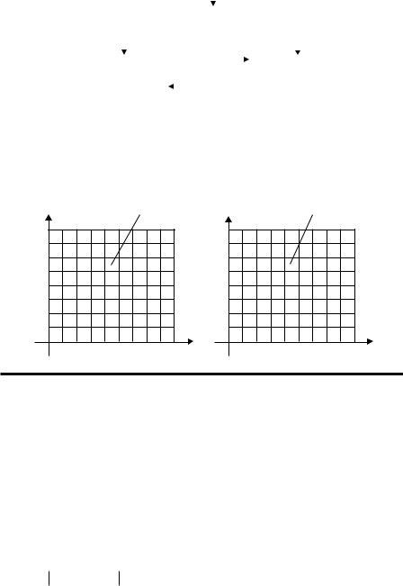
Figure 6.9 Paired comparison of scan patterns.

comparison, each of the two neighboring scans is displayed in a 256-by-256 gridbased color panel, in which coordinates x and y correspond to the third and fourth bytes of the destination IP addresses in a class B network. As shown in Figure 6.9, using the extracted fingerprints c(i,j) and c′(i,j) for each grid in the paired scans, we can obtain the similarity between them. To quantitatively compare paired scans, Muelder et al. (2005) proposed three wavelet scalograms for each

scan, Dk = (dk,1, …, dk,2n −k ), Sk = (sk,1, …, sk,2n −k ), and σk = (∑Sk2n−k ), for the given scan data series D0 = (d0,1, …, d ) and 0 < k < n. They also recommended

several functions for the calculation of dk,1 and sk,1, e.g., dk,i = |dk−1,i + dk−1,i+1|∙2 and sk,i = dk −1,i − dk −1,i +1 2. Furthermore, the wavelet similarity between scans can

be measured using distance functions, such as Euclidean distance. Based on the

156    Data Mining and Machine Learning in Cybersecurity

scalogram similarity between paired scans, scan clusters can be generated in an overview graph (Figure 6.9). The clustered scans can aid cyber administrators to investigate attack sources through the local analysis of an individual scan in the same cluster.

In experiments, Muelder et al. collected real-world scan data from the cyberinfrastructure at Lawrence Livermore National Lab (LLNL). Each scan data contained time information and the destination address. They showed a number of clustering results for visualization. However, no performance evaluation has been provided for recognition accuracy and speed. In addition, the recognition is performed by human visualization, and automatic scan comparisons have not been investigated.

6.4Other Scan Techniques with Machine-Learning Methods

As we explained in Study Application 3, SNORT and BRO used rule-based threshold techniques in scan detection. These techniques have low effectiveness and efficiency. Leckie and Kotagiri (2002) built a probabilistic system based on the Bayesian model. Using conditional probability, they estimated the likelihood of source IPs scanning the destination services on targets.

Robertson et al. (2003) assigned a score to each source IP according to the account of its failed connection with the destinations. If the score was greater than a given threshold, the source IP was detected as a scanner. They also developed a peer-center surveillance detection system to strengthen the scan detection ability even if they received no response in scanning. Yegneswaran et al. (2003) investigated the daily activities of source IPs in coordinated scans and found that there was no locality among the scanning activities across the source IPs. They also applied the information-theoretic approach to investigate the possibility of using the traffic information between networks to detect attackers. Conti and Abdullah (2004) developed a visualization method to detect coordinated scans and attack tools in normal traffic flows. Although they had not provided a clear visualization, results show that this method detected the distribution of coordinated scans.

6.5 Summary

In this chapter, we have investigated popular scan and scan detection techniques. Normally, scans represent the characteristics of attackers and scans can lead to potential attacks in similar scanned destinations across networks. Thus, scan detection can help users protect cyberinfrastructures from attacks.

Traditional scan detection methods use rule-based thresholding. These techniques normally result in a low detection rate and an unacceptable FAR, the same problem as occurs in most of the anomaly detection systems. The GrIDS approach constructs a hierarchical network graph, which can be helpful for cyber

Machine Learning for Scan Detection    157

administrators to investigate the causal relations between network activities, especially in large-scale networks. The aggregation of information in networks facilitates scan detection in multiple hosts or in groups of hosts, and consolidates its scalability to recognize the global scan patterns.

SPICE and SPADE detect stealth scans, especially when scans are evasive and in small-sized time windows normally used in traditional methods such as SNORT, BRO, and GrIDS. Using BN and clustering methods, SPICE and SPADE can detect slow scans at a high-detection rate and a low FAR. The TRW approach is used to detect scans quickly while solving effectiveness and efficiency problems in SNORT and BRO. This approach works as the gold standard for many innovative scan detection approaches. In comparison with TRW, it was found that SPICE needs days or weeks to collect packets and find clusters and correlations. The running time is longer, and the computation is more complex than with TRW. Simon et al. have demonstrated that expert rule-based data-mining techniques can outperform TRW in scan detection in terms of accuracy and coverage. Other machine-learning methods can be introduced into the workflow to improve the scan detection results. Gates et al. integrated logistic regression and feature extraction and selection into one module and found the hybrid scan detection result was similar to TRW.

To the best of our knowledge, most of the clustering and classic machinelearning methods have not been explored in scan detections. This lack of exploration can be because the dynamic and huge-scale network flows require an effective, real-time responsive learning ability in detection systems. Besides accuracy, scan detection needs sufficient coverage and scalability in large-scale cyberinfrastructures. As shown in Application Study 6, machine-learning classification and clustering methods can be integrated in both the global and local viewing of scan patterns in networks. This global and local viewing of scan patterns can potentially solve coverage and scalability problems. Meanwhile, the research could potentially extend to the further analysis of scan patterns, which will aid cyber administrators in launching preventive measures for potential attacks.

References

Braynov, S. and M. Jadliwala. Detecting malicious groups of agents. In: Proceedings of the First IEEE Symposium on Multi-Agent Security and Survivability, Philadelphia, PA, 2004.

Cohen, W.W. Fast effective rule induction. In: Proceedings of the 12th International Conference on Machine Learning, San Mateo, CA, 1995.

Conti, G. and K. Abdullah. Passive visual fingerprinting of network attack tools. In: Proceedings of 2004 CCS Workshop on Visualization and Data Mining for Computer Security, Washington, DC, 2004, pp. 45–54.

Gates, C., J.J. McNutt, J.B. Kadane, and M.I. Kellner. Scan detection on very large networks using logistic regression modeling. In: Proceedings of the 11th IEEE Symposium on Computers and Communications (ISCC), Cagliari, Sardin, 2006.