125 Кібербезпека / 4 Курс / 3.1_3.2_4.1_Захист інформації в інформаційно-комунікаційних системах / Лiтература / [Sumeet_Dua,_Xian_Du]_Data_Mining_and_Machine_Lear(BookZZ.org)

98    Data Mining and Machine Learning in Cybersecurity

They define a cosine distance metric for the KNN application as follows:

where

X denotes testing program

Yj denotes the jth training program

si denotes a system call occurring in both X and Yj

∙X ∙ and ∙Yj ∙ denote the norm calculated using Euclidean distance

The experiments were performed using BSM audit data found in the 1998 DARPA intrusion detection evaluation data sets. First, the authors chose 3556 normal programs and 49 distinct system calls in 1 simulation day load for the training phase. Second, they scanned the test audit data for programs to measure the distance using Equation 4.4. Third, the distances were ranked, corresponding to the top K scores for K nearest neighbors for this test audit data. A threshold was applied on the averaged K distances as a cutoff of anomaly detection. Various thresholds and K values were tested in experiments, such that the best performance of the KNN algorithm could be obtained in ROC curves. They reported that the empirical result showed that KNN algorithms detected 100% of the attacks while keeping a FPR at 0.082% with k = 5 and threshold = 0.74.

This method seems to offer computational advantages over methods that seek to characterize program behavior with short sequences of system calls and generate individual program profiles.

4.4.5 Hidden Markov Model

HMM considers the transition property of events in cyberinfrastructure. In anomaly detection, HMMs can effectively model temporal variations in program behavior (Warrender et al., 1999; Qiao, 2002; Wang et al., 2006). To apply HMM in anomaly detection, we begin with a normal activity state set S and a normal observable data set of O, S = {s1, …, sM}, and O = {o1, …, oN}. Given an observation sequence Y = ( y1, …, yT), the objective of HMM is to search for a normal state sequence of X = (x1, …, xT), which has a predicted observation sequence most similar to Y with a probability for this examination. If this probability is less than a predefined threshold, we declare that this observation indicates an anomaly state.

Application Study 6: Application of HMM Approach for Anomaly Detection (Table 1.3, C.8)

In 1999, Warrender et al. performed studies on various publicly available system call data sets from nine programs, such as MIT LPR, and UNM LPR. They suggested

Machine Learning for Anomaly Detection    99

that this number roughly corresponded to the number of system calls used by the program. For instance, they implemented 40-state HMMs for many of the programs because 40 system calls composed those programs. The states were fully connected; transitions were allowed from any state to any other state. Transitions and probabilities were initialized randomly, while occasionally, some states were predetermined with knowledge. Then, the Baum-Welch algorithm was applied to build the HMM using training data, and the Viterbi algorithm was implemented on the HMM to find the state sequence of system calls. They assumed that in a good HMM, normal sequences of system calls require only likely transitions and outputs, while anomalous sequences have one or more system calls that require unusual transitions and outputs. Thus, each system call was tested for tracking unusual transitions and outputs. They selected the same threshold, which varied from 0.0000001 to 0.1, for transitions and outputs.

The experiments showed that HMM could detect anomaly data quickly and at a lower mismatch rate. However, HMM training needs multiple passes through the training data, which takes a great deal of time. HMM training also requires extensive memory to store transition probabilities during training, especially for long sequences. We leave the calculation of the required memory size to the reader. Please make further analysis on how to improve the efficiency of HMM in this application.

4.4.6 Kalman Filter

Anomaly detection of network traffic flow is capable of raising an alarm and directing the cyber administrators’ attention to the particular original-destination flows. Further analysis and diagnosis can trigger measurements to isolate and stop the anomalies. However, most cybersecurity solutions focus on traffic patterns in one link. Any data flow can transverse multiple links along its path, and anomaly information in the flow may be identified in any route to its destination. Thus, the identification of the data flow in all links in an enterprise information infrastructure will be helpful for the collection of anomaly detection in the network.

A traffic matrix has entries of average workflow from given original nodes to other destination nodes in the given time intervals. These nodes can be computers or routers. As the entries in traffic matrix are dynamic and evolve over time, those entries can be estimated on the recent measurements after a time interval. The entries can be predicted before these recent measurements. The significant difference between the recent estimations and recent predictions will alert a cybersecurity program of an anomalous behavior. Thus, we focus on modeling the dynamic traffic matrix, which consists of all pairs of origin-destination (OD) flows in a cyberinfrastructure. By adapting the notations in Equation 3.14 in Section 3.4.6.1 to the notations in networks, we describe the implementation of Kalman filter in anomaly detection. As no control is involved in cyberinfrastructure, the equation xt = At xt−1 + wt, wt N(0, Q t ) relates network state xt–1 to xt with the state transition

100    Data Mining and Machine Learning in Cybersecurity

matrix At and noise process wt. Equation yt = Ht xt + vt, vt N(0, Rt) correlates yt, the link counts vector at time t, to xt, the OD flows. Here, we organize OD flows as a vector account for traffic traversing the link. Ht denotes whether an OD flow (row) traverses a link (column).

As displayed in Figure 2.6, the Kalman filter solves the estimation problem in two steps: prediction and estimation. We do not describe the details of the inference process; interested readers should refer to Soule et al. (2005). If we obtain the prediction ˆxt|t − 1, the error in the prediction of link values is εt = yt − Htˆxt|t − 1. Furthermore, we obtain the residual ςt = ˆxt|t − ˆxt|t − 1 = Ktεt, where Kt is the Kalman gain in Figure 2.6. This residual presents the information variation incurred by the new measurement in the network flow. It consists of errors from the network traffic system and anomalies in the infrastructure. Based on this analysis, further anomaly detection schemes can be developed to help network administrators make security decisions.

Application Study 7: Application of Kalman Filter for Anomaly Detection (Table 1.3, C.7) (Soule et al., 2005)

Soule et al. (2005) introduced an approach for anomaly detection for large-scale networks. They attempted to recognize traffic patterns by analyzing the traffic state using a network-wide view. A Kalman filter is used to filter out the “normal” traffic state by comparing the predictions of the traffic state to an inference of the actual traffic state. Then, the residual filtered process is examined for anomalies.

4.4.7 Unsupervised Anomaly Detection

Supervised detection methods use attack-free training data. However, audit data labels are difficult to obtain in real-world network environments. This problem also occurs in signature detection, due to the challenges in manually classifying the small number of attacks in the huge amount of cyber information. Moreover, with the changing network environment or services, patterns of normal traffic will change. The differences between the training and actual data can lead to high FPRs of supervised IDSs.

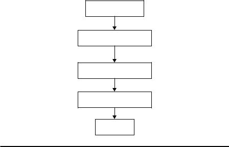
To address these problems, unsupervised anomaly detection emerges to take unlabeled data as input. Unsupervised anomaly detection aims to find malicious information buried in cyberinfrastructure even without prior knowledge about the data labels and new attacks. Subsequently, unsupervised anomaly detection methods rely on the following assumptions: normal data covers majority while anomaly data are minor in network traffic flow or audit logs; anomaly data points or normal data points are similar in their identity groups while statistically different between groups. We define anomaly detection as an imbalanced learning problem and consider that normal and anomaly data can be clustered. Thus, most of the solutions to unsupervised anomaly detection are clustering-based anomaly/outlier detection techniques. As shown in Figure 4.5, a typical unsupervised anomaly detection

Machine Learning for Anomaly Detection    101

Data collection

Data preprocessing

Unsupervised ML

Anomaly detection

Decision

Figure 4.5 Workflow of unsupervised anomaly detection.

system consists of five steps. The first and fifth steps are similar to the other anomaly detection systems. The second, third, and fourth steps contain two assumptions that require the modification and improvement of classic machine-learning methods for cyber anomaly detection. The data processing step will modify the training and testing data so that unsupervised methods can be applied on the valid data based on the above two assumptions. The unsupervised machine-learning methods must be designed for the imbalanced data. The machine-learning results can be used for detection only after labeling the groups, which require intelligent control of some parameters for optimal detection.

4.4.7.1 Clustering-Based Anomaly Detection

Chandola et al. (2006) categorized clustering-based techniques into three groups according to assumptions. Such categorization method is similar to assigning specific patterns or characteristics to the groups of normal and anomalous data. As with KNN, we categorize clustering-based anomaly detection into two groups: distance-based clustering and density-based clustering. The first group includes k-means clustering (Portnoy et al., 2001; Jiang et al., 2006), EM (Eskin, 2000; Traore, 2008), and SOM (Sarasamma and Zhu, 2006). The second group includes CLIQUE and MAFIA (Leung and Leckie, 2005). We focus on the first group because, according to our knowledge, the second group has fewer research results, and does not have as good anomaly detection results as the first group. For further information about density-based methods, such as CLIQUE and MAFIA, and

102    Data Mining and Machine Learning in Cybersecurity

their applications, readers should consult Leung and Leckie (2005) and Agrawal et al. (1998) for further reading.

The most deployed distance-based clustering method is adapted from k-means clustering (see Section 2.1.1). Without defining K in these algorithms, the clustering hyper-spheres are constrained by a threshold r. Given data set X = {x1, …, xm} and cluster set C = {C1, …, CK}, distance metric dist(xi, Cj) measures the closeness between data point xi, i = 1, …, m, and cluster Cj. To implement distance-based clustering, follow the steps below:

Step 1. Initialize cluster set C = {C1, …, CK}.

Step 2. Assign each data point xi in X to the closest cluster C *, C * {C1, …, CKÕ}, if dist(xi, C *) ≤ r ; or creation of new cluster C′ for this data point, and update the cluster set C.

Step 3. Iterate until all data points are assigned to a cluster.

In the above steps, the most employed distance metric is Euclidean distance. If we choose the distance between a data point xi and cluster Cj to measure dist(xi, Cj), the above algorithm will be similar to k-means clustering, except we will have an additional constraint r for the clustering threshold. As all training data are unlabeled, we cannot determine which clusters belong to normal or anomaly types. Each cluster may include mixed instances of normal data and different types of attacks. As we assume that normal data over-number anomaly data, generally the clusters that constitute more than a percentage α of the training data set are labeled as “normal” groups. The other clusters are labeled as “attack.”

As we implicitly determine abnormal clusters by the size of these classes, some small-sized normal data groups can be misclassified as anomaly clusters especially when we have multi-type normal data. We recommend readers further analyze and explore the solutions to this problem. Meanwhile, threshold r also affects the result of clustering. When r is large, the cluster number will decrease; when r is small, the cluster number will increase. The selection of r is dependent on the knowledge of the normal data distribution. For instance, we know statistically it should be greater than the intra-cluster distance and smaller than the inter-cluster distance. Jiang et al. (2006) selected r by generating the mean and standard deviation of distances between pairs of a sample data points from the training data set.

Once the training data have been clustered and labeled, testing data can be grouped according to their shortest distance to any cluster in the cluster set.

Application Study 8: Application of Clustering for Anomaly Detection

Portnoy et al. (2001) applied the clustering anomaly detection method on the DARPA MIT Knowledge Discovery and Data Mining (KDD) Cup 1999 data set. This data set recorded 4,900,000 data points with 24 attack types and normal activity in the background. Each data point is a vector of extracted feature values from the connection record obtained between IP addresses during simulated intrusions.

Machine Learning for Anomaly Detection    103

The authors performed CV in training and testing. The entire KDD data set was partitioned into 10 subsets. The subsets containing only one type of attacks or full of attacks were removed, such that only four subsets were left for CV. Then, they filtered the training data sets from KDD data for attacks such that the attack data and normal data had a proportion about 1:99 in the resulting training data set.

Before training and testing phases, the authors evaluated the performance using ROC (FP-TP). They ran 10% of the KDD data to measure the performance when choosing the sensitive parameters: threshold r and percentage 1 − α. They selected r = 40 and α = 0.85 after balancing between TP and FP in ROC for achieving the higher TP and acceptable FP.

Finally, training and testing were performed several times with different selections of the combinational subsets for training and testing. Clustering with unlabelled data resulted in a lower detection rate for attacks than clustering with supervised learning. However, unlabeled data can potentially detect unknown attacks through an automated or semi-automated process, which will allow cyber administrators to concentrate on the most likely attack data.

4.4.7.2 Random Forests

Random forests have been employed broadly in various applications, including multimedia information retrieval and bioinformatics. The random forests algorithm has better predication accuracy and efficiency on large data sets in highdimensional feature space. Network traffic flow has such data characteristics such that random forest algorithms are applied (Zhang and Zulkernine, 2006; Zhang, 2008) to detect outliers in data sets of network traffic without attack-free training data. In the framework, the reported results show that the proposed approach is comparable to previously reported unsupervised anomaly detection approaches.

As introduced in Section 2.1.1.9, the accuracy of random forests depends on the strength of the individual tree classifiers and a measure of the dependence between them. The number of randomly selected features at each node is critical for the estimated quality of the above measures.

Consequently, in building the network traffic model, two important parameters must be selected: the number of random features to split the node of trees (Nf), and the number of trees in a forest (Nt). The combinational values of these two variables are selected, corresponding to the optimal prediction accuracy of the random forests.

In the detection process, random forests use proximity measure between the paired data points to find outliers. If a data point has low proximity measures to all the other data points in a given data set, it is likely to be outlier. Given a data set X = {x1,…, xn}, enquiry

data point xenquiry X, and all the other data in class Cj, xj Cj, the average proximity between data point xenquiry, and all the other data points xj Cj are defined as,

104    Data Mining and Machine Learning in Cybersecurity

The degree of a data point xenquiry to be an outlier of class Cj is represented as

We can set a threshold for the above equation so that any xenquiry X will be detected as an outlier. In the above, |Cj| and |X| denote the number of data points

in class Cj and X, respectively.

The proximity between xenquiry and xj Cj, prox2(xenquiry , xj), is accumulated by one, when both data points are found in the same leaf of a tree. The final sum-

mation result should be divided by the number of trees to normalize the results. Following the above equations, we can obtain proximity, and the degree of an outlier in any class for each data point extracted from a network traffic data set. Moreover, the decision can be made using the threshold.

Application Study 9: Application of Random Forests for Anomaly Detection

Zhang and Zulkernine (2006) applied the random forest algorithm to the DARPA MIT KDD Cup 1999 data set. They selected five services as pattern labels for a random forests algorithm, including ftp, http, pop, smtp, and telnet. Since services appear in any network traffic flow, this labeling process is automatic, and the original labels of attack types or “normal” are removed. Four groups of data sets were generated by combining normal data and attack data at the ratio of 99:1, 98:2, 95:5, and 90:10. A total of 47,426 normal traffic flow data were selected from ftp, pop, telnet, 5% http, and 10% smtp normal services.

The authors evaluated the performance of the system using ROC. They reported a better detection rate while keeping the FP rate lower than in other unsupervised anomaly detection systems presented by Portnoy et al. (2001) and Leung and Leckie (2005). However, they indicated that the detection performance over minority attacks was much lower than that of majority intrusions. They improved the detection system by using random forests in the hybrid system of misuse detection and anomaly detection. We discuss this problem in Chapter 5.

4.4.7.3 Principal Component Analysis/Subspace

As we discussed in Section 3.4.6, anomaly detection in OD flows is challenging due to the high-dimensional features and noisy and large volumes of streaming data. This problem becomes more difficult as Internet links are developed and integrated to more complex and faster networks. Network anomaly detection using dimensionality reduction techniques has received much attention recently. In particular, network-wide anomaly detection based on PCA has emerged as a powerful method for detecting a wide variety of anomalies. PCA has demonstrated its ability in finding correlations across multiple links in network-wide analysis (Lakhina et al., 2004a,b) and detecting a wide variety of anomalies (Lakhina, 2004).

Machine Learning for Anomaly Detection    105

Let matrix Y denote the network traffic data in space d × n, where each row presents a data point, e.g., observation at a time point, and each column presents a link in network. As discussed in Section 1.3.2.5, PCA can explore the intrinsic principle dimensionality and present the variance of data along these principle dimensions such that the variability of data can be captured in a lower dimensionality. Meanwhile, traffic on different links is dependent, and link traffic is the superposition of OD flows. Lakhina et al. (2004a,b) showed that, in a 40-link network, three-to-four principal components could capture the majority of variance in the link time-series data.

Using the PCA method described in Section 1.3.2.5, we can project network traffic flow data in matrix Y to any principle component (direction) vi by Y · vi (eigenvalue). The value of Y · vi indicates the significance of network flows captured in the ith principal component. Given observations in matrix Y are time-series network flow, principal component vi presents the ith strongest temporal trend in the whole network flows. As normal data dominate network traffic, we can assign the top principal flow in normal group, and the remaining flows as anomalies.

Let S denote the space spanned by the first p principal components and S denote

the remaining principal components. Then, each traffic flow y can be decomposed

−

into two subspaces: normal traffic vector y and anomaly traffic vector y. Using

the top p principal components as columns, we obtain a matrix Q = [v1, …, vp ].

−

Next, we project data Y onto normal space S and anomaly space S by y = QQTy, andy = (1 − QQT )y · y can measure the sudden anomaly behavior in network OD flow. Moreover, we can use this decomposition to detect the time of the anomaly flow, identify the anomaly source and destination, and quantify the size of the anomaly.

Assuming the network-traffic flow data follows multivariate Gaussian distri- bution, a threshold εβ2 can be obtained using statistical estimation. If y 2 ≤ εβ2,

we say this network traffic flow y is normal at the 1 − β confidence level. Lakhina et al. (2004a,b) applied the Q-statistic test using the results from Jackson and Mudholkar (1979).

PCA-based subspace methods have been explored in a number of research reports (Lakhina, 2004; Lakhina et al., 2004a,b, 2005; Li, 2006; Ringberg et al., 2007) because of their effective ability to diagnose network traffic anomalies in an entire cyber system. However, it has also been found that tuning PCA to operate effectively is difficult and requires more robust techniques than have been presented thus far.

The Ringberg et al. (2007) study identified and evaluated four challenges associated with using PCA to detect traffic anomalies; e.g., sufficient large anomalies can contaminate the normal subspace. Robust statistical methods are developed to solve the sensitivity problems. Moreover, Li et al. (2006) showed how to use random aggregations of IP flows (i.e., sketches) for a more precise identification of the underlying causes of anomalies. They presented a subspace method to combine traffic sketches to detect anomalies with a high accuracy rate and to identify the IP flows(s) that are responsible for the anomaly.

106    Data Mining and Machine Learning in Cybersecurity

Table 4.3 Data Sets Used in Lakhina et al. (2004a)

Source: Lakhina, A. et al., Characterization of network-wide anomalies in traffic flows, in: Proceedings of the 4th ACM SIGCOMM Conference on Internet Measurement, Taormina, Sicily, Italy, 2004a, pp. 201–206. With permission.

Application Study 10: Application of PCA/Subspace for Anomaly Detection (Table 1.3, C.4 and C.11)

Lakhina et al. (2004a,b) collected three network-traffic data sets from two backbone networks: Sprint-Europe and Abilene. As shown in Table 4.3, the authors aggregated packets into flows and aggregated traffic-flow byte counts, which they then divided into bins of 10 min to sample both Sprint and Abilene data sets.

Because the true anomalies have to be identified in data sets before the quality of the estimated anomalies of the proposed PCA-based subspace method can be determined, the authors employed an exponential weighted moving average and Fourier scheme on the OD flow level to capture the volume anomalies. Then, they evaluated the PCA-based subspace method in diagnosing the above networks using the detection rate (TP) and false-alarm rate (FP), and the diagnosis effectiveness in the event that the time and location of anomalies varied. The results showed that PCA-based subspace consistently diagnoses the largest volume anomalies with a higher detection rate and a lower FAR.

4.4.7.4 One-Class Supervised Vector Machine

As shown in Section 3.4.3, a standard SVM is a supervised machine-learning method, which requires labeled data for training the classification model. SVM has been adapted into an unsupervised machine-learning method in Jackson and Mudholkar (1979). The one-class SVM attempts to separate the data from the origin with a maximum margin by solving the following quadratic optimization: