

Velocity and Coordinate by Integration
When
varies
with time, we can use the relation
![]() to
find the velocity
as
a function of time if the position
is a given function of time. Similarly, we can use
to
find the velocity
as
a function of time if the position
is a given function of time. Similarly, we can use
![]() to find the acceleration
as a function of time if the velocity
to find the acceleration
as a function of time if the velocity
![]() is
a given function of time.
is
a given function of time.
We can also reverse this process. Suppose is known as a function of time; how can we find as a function of time? To answer this question, we first
Fig.3 The area under a velocity-time graph equals the displacement |
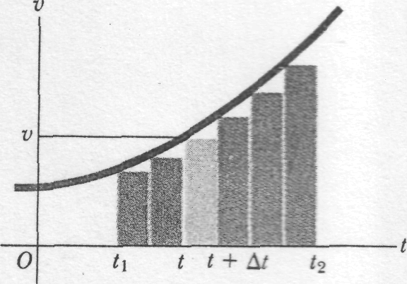
consider a
graphical approach. Figure 3 shows a velocity-versus-time curve for a
situation where the acceleration (the slope of the curve) is not
constant but increases with time. Considering the motion during the
interval between times
![]() and
and
![]() ,
we
divide this total interval into many smaller intervals, calling a
typical one
.
Let
the velocity during that interval be
.
Of
course, the velocity changes during
,
but
if the interval is very small, the change will also be very small.
This displacement during that interval, neglecting the variation of
,
is
given by
,
we
divide this total interval into many smaller intervals, calling a
typical one
.
Let
the velocity during that interval be
.
Of
course, the velocity changes during
,
but
if the interval is very small, the change will also be very small.
This displacement during that interval, neglecting the variation of
,
is
given by
![]() .
.
This
corresponds graphically to the area of the shaded strip with height
and
width
,
that
is, the area under the curve corresponding to the interval
.
Since
the total displacement in any interval (say,
to
)
is
the sum of the displacements in the small subintervals, the total
displacement is given graphically by the total
area
under the curve between the vertical lines
and
.
In
the limit, when all the
become
very small and their number very large, this is simply the integral
of
(which
is in general a function of
)
from
and
.
Thus
is the position at time
and
![]() the
position at time
:
the
position at time
:
 (2-14)
A similar
analysis with the acceleration-versus-time curve, where
is
in general a function of
,
shows
that if
is
the velocity at time
and
![]() the
velocity at time
,
the
change in velocity
the
velocity at time
,
the
change in velocity
![]() during
a small time interval
is
approximately equal to
during
a small time interval
is
approximately equal to
![]() ,
and
the total change in velocity (
,
and
the total change in velocity (![]() )
during
the interval
)
during
the interval
![]() is given by
is given by

Or,
finally,
![]() .
.
Exercises
1. Velocity
of a body, moving in viscous medium, is given by the equation
![]() ,
where
,
where
![]() - initial velocity,
- initial velocity,
![]() - constant. What are the distance and acceleration as function of
time?
- constant. What are the distance and acceleration as function of
time?
2. A
particle moves along a straight line with velocity
![]() ,
where
is constant. If at time
,
where
is constant. If at time
![]() the distance, traveled the particle was
the distance, traveled the particle was
![]() ,
determine: (a) dependence of speed and acceleration on time (
,
determine: (a) dependence of speed and acceleration on time (![]() and
and
![]() )
)
3. (a) If
particle’s acceleration is given by
![]() ,
(where
is in meter/second2
and
in seconds), what its velocity at
?
(b) What is its coordinate at
s?
,
(where
is in meter/second2
and
in seconds), what its velocity at
?
(b) What is its coordinate at
s?
4-8 Relative Motion in One Dimension
Suppose you see a duck flying north at, say, 30 km/h. To another duck flying alongside, the first duck seems to be stationary. In other words, the velocity of a particle depends on the reference frame of whoever is observing or measuring the velocity. For our purposes, a reference frame is the physical object to which we attach our coordinate system. In everyday life, that object is the ground. For example, the speed listed on a speeding ticket is always measured relative to the ground. The speed relative to the police officer would be different if the officer were moving while making the speed measurement.
|
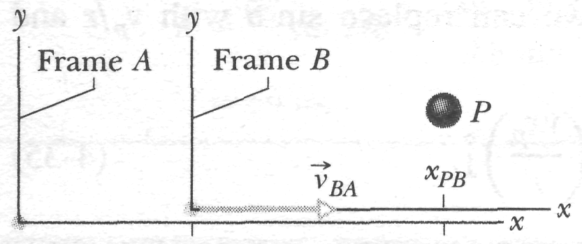
Fig.
4-20
Alex
(frame A)
and
Barbara (frame
B)
watch
car P,
as
both В
and
P
move
at different velocities along the common
axes of the two frames. At the
instant shown,
![]() is
the coordinate of
В
in
the A
frame.
Also, P
is
at coordinate
is
the coordinate of
В
in
the A
frame.
Also, P
is
at coordinate
![]() in
the В
frame
and coordinate
in
the В
frame
and coordinate
![]() in
the A
frame.
in
the A
frame.
Suppose that Alex (at the origin of frame A) is parked by the side of a highway, watching car P (the "particle") speed past. Barbara (at the origin of frame B) is driving along the highway at constant speed and is also watching car P. Suppose that, as in Fig. 4-20, they both measure the position of the car at a given moment. From the figure we see that
![]() (4-38)
(4-38)
The
equation is read: "The coordinate
![]() of
P
as
measured by A
is equal to the
coordinate
of
P
as
measured by A
is equal to the
coordinate
![]() of
P
as
measured by В
plus the
coordinate
of
В
as
measured by A."
Note
how this reading is supported by the sequence of the subscripts.
Taking the time derivative of Eq. 4-38, we obtain
of
P
as
measured by В
plus the
coordinate
of
В
as
measured by A."
Note
how this reading is supported by the sequence of the subscripts.
Taking the time derivative of Eq. 4-38, we obtain
![]()
Or
(because
![]() )
)
![]() (4-39)
(4-39)
This
equation is read: "The velocity
![]() of P
as
measured by A
is equal to the
velocity
of P
as
measured by A
is equal to the
velocity
![]() of
P
as
measured by В
plus the
velocity
of
P
as
measured by В
plus the
velocity
![]() of
В
as
measured by A."
The
term
is
the velocity of frame В
relative
to frame A.
(Because
the motions are along a single axis, we can use components along that
axis in Eq. 4-39 and omit overhead vector arrows.)
of
В
as
measured by A."
The
term
is
the velocity of frame В
relative
to frame A.
(Because
the motions are along a single axis, we can use components along that
axis in Eq. 4-39 and omit overhead vector arrows.)
Here we consider only frames that move at constant velocity relative to each other. In our example, this means that Barbara (frame B) will drive always at constant velocity relative to Alex (frame A). Car P (the moving particle), however, may speed up, slow down, come to rest, or reverse direction (that is, it can accelerate).
To relate an acceleration of P as measured by Barbara and by Alex, we take the time derivative of Eq. 4-39:
![]() (4-40)
(4-40)
Because is constant, the last term is zero and we have
![]() .
In
other words.
.
In
other words.
► Observers on different frames of reference (that move at constant velocity relative to each other) will measure the same acceleration for a moving particle.
4-9 Relative Motion in Two Dimensions
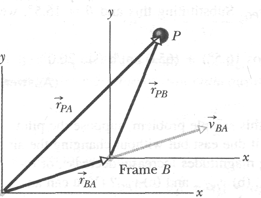
Now we turn from relative motion in one dimension to relative motion in two (and, by extension, in three) dimensions. In Fig. 4-21, our two observers are again watching a moving particle P from the origins of reference frames A and B, while В moves at a constant velocity relative to A. (The corresponding axes of these two frames remain parallel.)
Figure 4-21
shows a certain instant during the motion. At that instant, the
position vector of В
relative
to A
is
![]() .
Also,
the position vectors of particle P
are
.
Also,
the position vectors of particle P
are![]() relative
to A
and
relative
to A
and
![]() relative
to B.
From
the arrangement of heads and tails of those three position vectors,
we can relate the vectors with
relative
to B.
From
the arrangement of heads and tails of those three position vectors,
we can relate the vectors with
![]() (4-41)
(4-41)
|
The plane
has velocity
![]() relative
to the wind, with an airspeed (speed relative to the wind) of 215
km/h, directed at angle
south
of east. The wind has velocity
relative
to the wind, with an airspeed (speed relative to the wind) of 215
km/h, directed at angle
south
of east. The wind has velocity
![]() relative
to the ground, with a speed of 65.0 km/h, directed 20.0° east of
north. What is the magnitude of the velocity
relative
to the ground, with a speed of 65.0 km/h, directed 20.0° east of
north. What is the magnitude of the velocity
![]() of
the plane relative to the ground, and what is 0?
of
the plane relative to the ground, and what is 0?
|
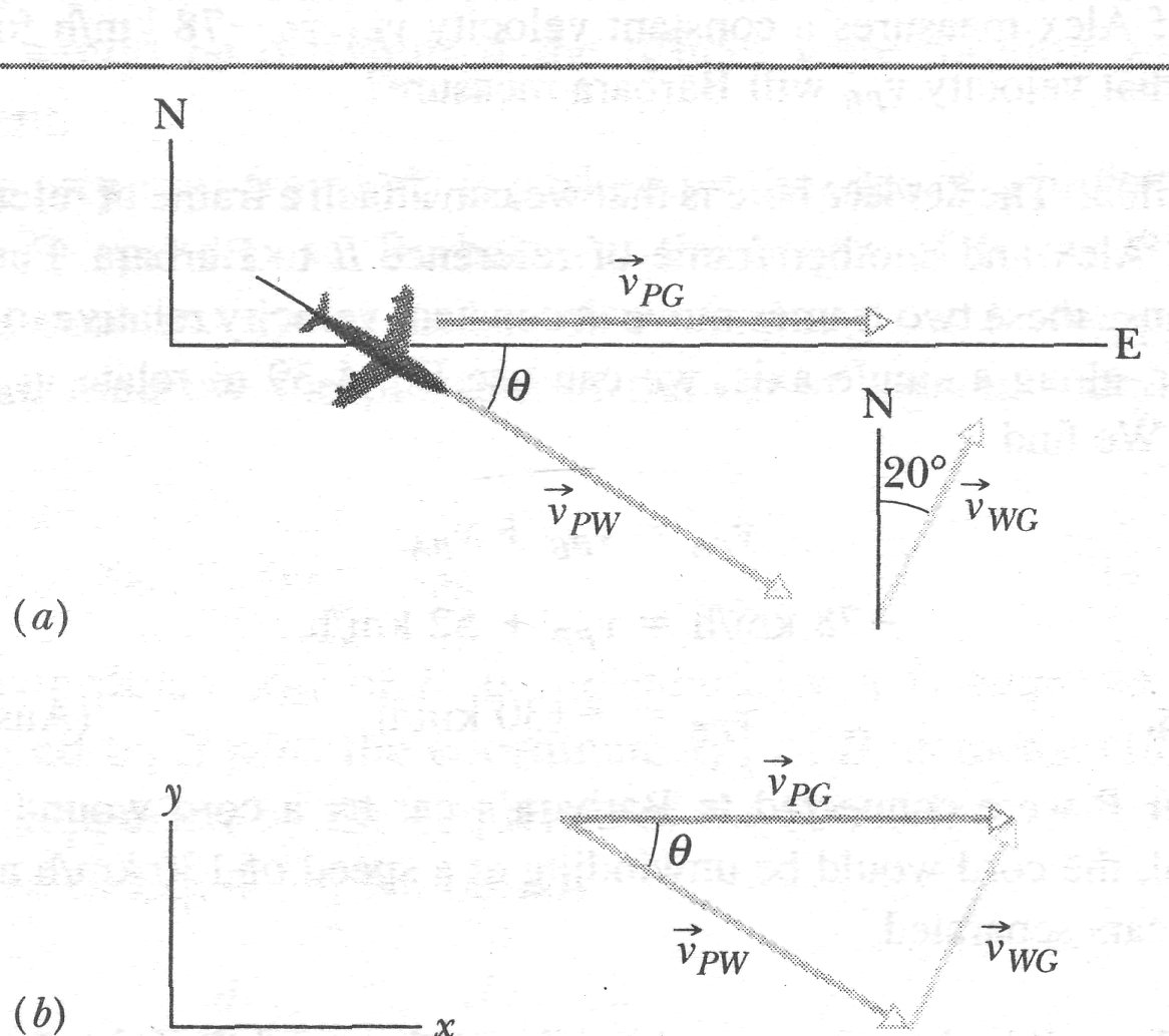
Fig. 4-21 Frame В has the constant two-dimensional velocity relative to frame A. The position vector of В relative to A is . The position vectors of particle P are relative to A and relative to B.
By taking the time derivative of this equation, of particle P we can relate the velocities and
![]()
By taking
the time derivative of this relation, we can relate the accelerations
![]() and
and
![]() of
the particle P
relative
to our observers. However, note that because
is
constant, its time derivative is zero. Thus, we get
of
the particle P
relative
to our observers. However, note that because
is
constant, its time derivative is zero. Thus, we get
As for one-dimensional motion, we have the following rule: Observers on different frames of reference that move at constant velocity relative to each other will measure the same acceleration for a moving particle.
 Sample
Problem 4-11
Sample
Problem 4-11
In Fig.
4-22a, a plane moves due east (directly toward the east) while the
pilot points the plane somewhat south of east, toward a steady wind
that blows to the northeast. SOLUTION:
The Key Idea is that the situation is like the one in Fig. 4-21.
Here the moving particle P
is
the plane, frame A
is
attached to the ground (call it
![]() ),
and frame В
is
"attached" to the wind (call it
),
and frame В
is
"attached" to the wind (call it
![]() ).
We
need to construct a vector diagram like that in Fig. 4-21 but this
time using the three velocity vectors.
).
We
need to construct a vector diagram like that in Fig. 4-21 but this
time using the three velocity vectors.
First construct a sentence that relates the three vectors:
![]()
![]()
We want the magnitude of the first vector and the direction of the second vector. With unknowns in two vectors, we cannot solve Eq. 4-44 directly on a vector-capable calculator. Instead, we need to resolve the vectors into components on the coordinate system of Fig. 4-226, and then solve Eq. 4-44 axis by axis (see Section 3-5). For the у components, we find
![]()
or
![]()
Solving for gives us
![]() (Answer)
(Answer)
Similarly, for the components we find
![]()
Here,
because
is
parallel to the
axis,
the component
![]() is
equal
to the magnitude
.
Substituting
this and
=16.5°,
we find
is
equal
to the magnitude
.
Substituting
this and
=16.5°,
we find
![]() (Answer)
(Answer)
A body
moves in a straight line
along
-axis.
Its distances
(in meter) from the origin is given by
![]() .
The
average
speed in the interval
to
.
The
average
speed in the interval
to
![]() second is
second is
(A) 5 m/s (B) -4 m/s
(C) 6 m/s (D) zero
A particle
moves along
-axis
in such a
way
that
its coordinate
vanes with time t
according
to
the expression
![]() .
The
acceleration of the particle
will
be
zero at
time
.
The
acceleration of the particle
will
be
zero at
time
(A)
![]() (B)
(B)
![]() (C)
(C)
![]() (D)
zero
(D)
zero
A particle
moves along a straight line,
such that its displacement
![]() (in metres). The velocity, when
the
acceleration is zero, is
(in metres). The velocity, when
the
acceleration is zero, is
(A) -12 m/s (B) -9 m/s (C) 3 m/s (D) 42 m/s
The
equation
![]() gives the variation of displacement
with
time. Which of the following is correct?
gives the variation of displacement
with
time. Which of the following is correct?
Velocity is proportional to time.
Velocity is inversely proportional to time.
Acceleration depends upon time.
Acceleration is constant.
A particle
moving along a straight
line has a velocity
m/s,
when
it cleared a distance of x
meters.
These two
are connected
by the relation
![]() .
When
its velocity
is l m/s, its acceleration (in m s-2)
is :
.
When
its velocity
is l m/s, its acceleration (in m s-2)
is :
(A) 2 (B) 7 (C) 1 (D) 0.5
If
![]() ,
where
x
is
the distance traveled
by the body kilometers,
while t
is
time in
seconds,
then
units of b
,
where
x
is
the distance traveled
by the body kilometers,
while t
is
time in
seconds,
then
units of b
(A) km/s (B) km·s (C) km/s2 (D) km·s2
An
acceleration
of a particle is increasing linearly
with time
as
![]() The
particle starts from
the origin with an initial
velocity
.
The
distance traveled by the particle in time
will be
The
particle starts from
the origin with an initial
velocity
.
The
distance traveled by the particle in time
will be
(A)
![]() (B)
(B)
![]() (C)
(C)
![]() (D)
(D)
![]()