Algorithms [Sedgewick, Robert]
.pdf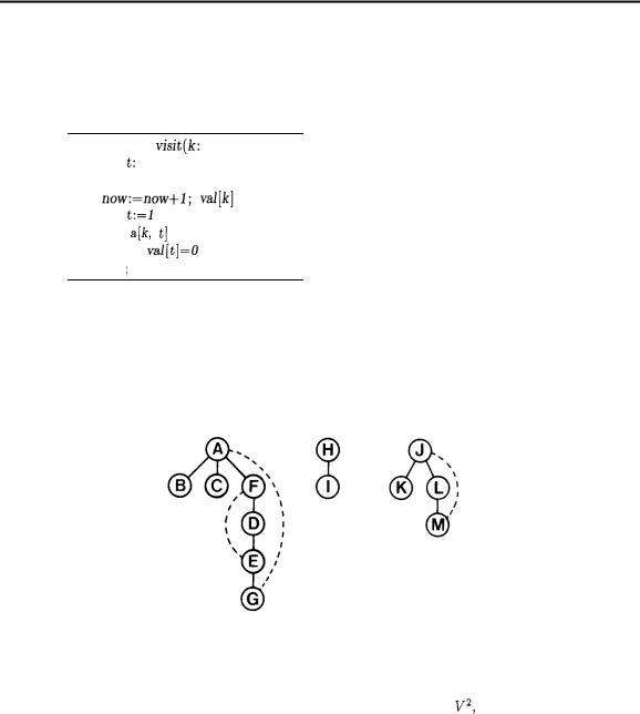

386 |
CHAPTER 29 |
ponents for later processing by more sophisticated algorithms.
Mazes
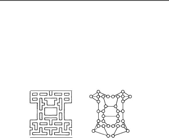
This systematic way of examining every vertex and edge of a graph has a distinguished history: depth-first search was first stated formally hundreds of years ago as a method for traversing mazes. For example, at left in the diagram below is a popular maze, and at right is the graph constructed by putting a vertex at each point where there is more than one path to take, then connecting the vertices according to the paths:
This is significantly more complicated than early English garden mazes, which were constructed as paths through tall hedges. In these mazes, all walls were connected to the outer walls, so that gentlemen and ladies could stroll in and clever ones could find their way out by simply keeping their right hand on the wall (laboratory mice have reportedly learned this trick). When independent inside walls can occur, it is necessary to resort to a more sophisticated strategy to get around in a maze, which leads to depth-first search.
To use depth-first search to get from one place to another in a maze, we use visit, starting at the vertex on the graph corresponding to our starting point. Each time visit “follows” an edge via a recursive call, we walk along the corresponding path in the maze. The trick in getting around is that we must walk back along the path that we used to enter each vertex when visit finishes for that vertex. This puts us back at the vertex one step higher up in the depth-first search tree, ready to follow its next edge.
The maze graph given above is an interesting “medium-sized” graph which the reader might be amused to use as input for some of the algorithms in later chapters. To fully capture the correspondence with the maze, a weighted


30. Connectivity
The fundamental depth-first search procedure in the previous chapter finds the connected components of a given graph; in this section we’ll examine related algorithms and problems concerning other graph connectivity
properties.
As a first example of a non-trivial graph algorithm we’ll look at a generalization of connectivity called biconnectivity. Here we are interested in knowing if there is more than one way to get from one vertex to another in the graph. A graph is biconnected if and only if there are at least two different paths connecting each pair of vertices. Thus even if one vertex and all the edges
touching |
it |
are removed, |
the graph is still connected. |
If it is important that |
a graph |
be |
connected for |
some application, it might |
also be important that |
it stay connected. We’ll look at a method for testing whether a graph is biconnected using depth-first search.
Depth-first search is certainly not the only way to traverse the nodes of a graph. Other strategies are appropriate for other problems. In particular, we’ll look at breadth-first search, a method appropriate for finding the shortest path from a given vertex to any other vertex. This method turns out to differ from depth-first search only in the data structure used to save unfinished paths during the search. This leads to a generalized graph traversal program that encompasses not just depth-first and breadth-first search, but also classical algorithms for finding the minimum spanning tree and shortest paths in the graph, as we’ll see in Chapter 31.
One particular version of the connectivity problem which arises frequently involves a dynamic situation where edges are added to the graph one by one, interspersed with queries as to whether or not two particular vertices belong to the same connected component. We’ll look at an interesting family of algorithms for this problem. The problem is sometimes called the “union-find” problem, a nomenclature which comes from the application of the algorithms
389
390 |
CHAPTER 30 |
to processing simple operations on sets of elements.
Biconnectivity
It is sometimes reasonable to design more than one route between points on a graph, so as to handle possible failures at the connection points (vertices). For example, we can fly from Providence to Princeton even if New York is snowed in by going through Philadelphia instead. Or the main communications lines in an integrated circuit might be biconnected, so that the rest of the circuit still can function if one component fails. Another application, which is not particularly realistic but which illustrates the concept is to imagine a wartime stituation where we can make it so that an enemy must bomb at least two stations in order to cut our rail lines.
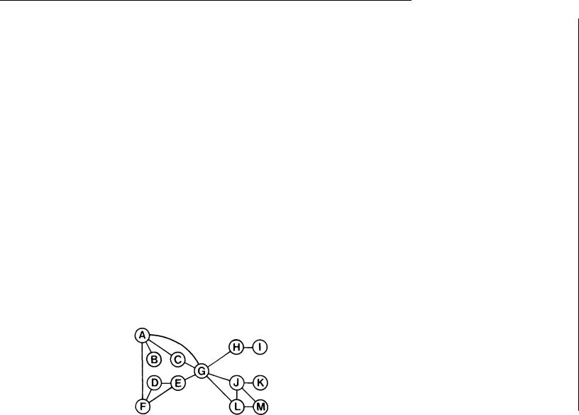
An articulation point in a connected graph is a vertex which, if deleted, would break the graph into two or more pieces. A graph with no articulation points is said to be biconnected. In a biconnected graph, there are two distinct paths connecting each pair of vertices. If a graph is not biconnected, it divides into biconnected components, sets of nodes mutually accessible via two distinct paths. For example, consider the following undirected graph, which is connected but not biconnected:
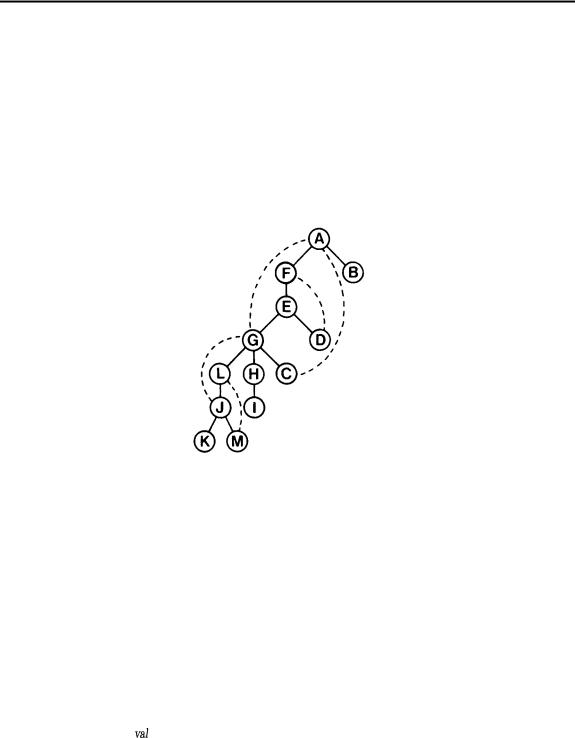
(This graph is obtained from the graph of the previous chapter by adding the edges GC, GH, JG, and LG. In our examples, we’ll assume that these fours edges are added in the order given at the end of the input, so that (for example) the adjacency lists are similar to those in the example of the previous chapter with eight new entries added to the lists to reflect the four new edges.) The articulation points of this graph are A (because it connects B to the rest of the graph), H (because it connects I to the rest of the graph), J (because it connects K to the rest of the graph), and G (because the graph would fall into three pieces if G were deleted). There are six biconnected components: ACGDEF, GJLM, and the individual nodes B, H, I, and K.
Determining the articulation points turns out to be a simple extension