

Phedotikov / 1 / FreeEnergy_27.01.08 / !Информация / Nikolo Tesla / Modern Physics For Engineers - Nikola Tesla
.pdfSCHRÖDINGER'S WAVE EQUATION
time-dependent form: |
|
|
|
|
|
|
|
|||||||||
|
|
|
|
|
|
|
K |
|
|
+ |
|
U |
= |
E |
||
- |
h2 |
|
¶2 Y( x, t ) |
+V Y (x, t ) = ih |
¶Y (x, t ) |
|||||||||||
2m |
|
|
|
|
¶x |
2 |
|
¶t |
||||||||
|
|
|
|
|
|
|
|
|
|
|
|
|||||
time-independent form: |
|
|
|
|
|
|||||||||||
|
|
|
|
|
|
|
|
|
||||||||
|
- |
h2 |
|
d 2y ( x) |
+V ( x )y( x) = Ey( x) |
|
||||||||||
|
|
|
dx2 |
|||||||||||||
|
|
2m |
|
|
|
|
|
|
|
|||||||
|
|
|
|
|
|
|
|
|
|
|
|
|
|
|
|
|
|
|
|
|
|
|
|
|
2 |
|
|
|
2 |
y( x) |
|
|
|
|
or |
- |
|
h |
|
|
d |
= E -V ( x) |
||||||||
|
2my ( x) |
d x2 |
||||||||||||||
|
|
|
|
|
|
|
|
|
|
|||||||
h = Planck's constant divided by 2π [J-s]
Ψ(x,t)
V = voltage; can be a function of space and time (x,t) m = mass [kg]
Two separate solutions to the time-independent equation have the form:
Aeikx + Be−ikx where k = 2m( E -V ) / h
or Asin (kx ) + B cos (kx )
Note that the wave number k is consistent in both solutions, but that the constants A and B are not consistent from one solution to the other. The values of constants A and B will be determined from boundary conditions and will also depend on which solution is chosen.
PROBABILITY
A probability is a value from zero to one. The probability may be found by the following steps:
Multiply the function by its complex conjugate and take the integral from negative infinity to positive infinity with respect to the variable in question, multiply all this by the square of a constant c and set equal to one.
∞
c2 ò−∞ F * F dx =1
Solve for the probability constant c.
The probability from x1 to x1 is: P = c2 òx2 F * F dx
x1
PROBABILITY OF LOCATION
Given the wave function: y( x, t )
find the probability that a particle is located between x1 and x2.
∞
Normalize the wave function: 2ò0 A2y2dx =1
with A known, find the probability: P = òx2 A2y2dx
x1
áxñ, áx2ñ EXPECTATION VALUES average value:
 x
x = ò−∞∞ y*( x) x y ( x)dx average x2 value:
 x2
x2  = ò−∞∞ y*(x ) x2 y(x )dx
pˆ MOMENTUM OPERATOR
An operator transforms one function into another function. The momentum operator is:
pˆ = -ih d dx
For example, to find the average momentum of a particle described by wave function ψ:
∞ |
ˆ |
∞ æ |
-ih |
d |
ö |
|
|
|
y÷ dx |
||
p = ò−∞ y* p y dx = ò−∞ y*ç |
dx |
||||
|
|
è |
|
ø |
|
Tom Penick tomzap@eden.com www.teicontrols.com/notes 12/12/1999 Page 11 of 22

SIMPLE HARMONIC MOTION
Examples of simple harmonic motion include a mass on a spring and a pendulum. The average potential energy equals the average kinetic energy equals half of the total energy. In simple harmonic motion, k is the spring constant, not the wave number.
spring constant k: |
w = |
k |
|
|
force: F = kx |
|
|
|||||||
m |
|
|
||||||||||||
|
|
|
|
|
|
|
|
|
|
|
|
|
|
|
potential energy V: |
V = |
1 |
kx2 |
|
|
|
|
|
||||||
|
|
|
|
|
|
|||||||||
|
|
2 |
|
|
|
|
|
|
|
|
|
|
||
Schrödinger Wave Equation |
|
|
d 2y |
|
= (a2 x2 -b)y |
|||||||||
for simple harmonic motion: |
|
|
2 |
|||||||||||
|
|
dx |
|
|
|
|
|
|||||||
where a2 = |
mk |
|
and b = |
|
2mE |
|
|
|
||||||
|
2 |
|
|
|
||||||||||
|
|
2 |
|
|
|
|
|
|
|
|
|
|
||
|
|
h |
|
|
|
|
h |
|
|
|||||
The wave equation solutions |
|
|
|
|
|
|
|
|
||||||
|
|
|
2 |
|
|
|||||||||
are: |
|
|
|
|
|
|
yn = Hn ( x)e−αx |
/ 2 |
|
|||||
where Hn(x) are polynomials of order n, where |
|
|
||||||||||||
n = 0,1,2,· · · and x is the variable taken to the power of n. |
||||||||||||||
The functions Hn(x) are related by a constant to the Hermite polynomial functions.
|
1 / 4 |
|
|
|
|
|
|
|
1 / 4 |
|
|
|
|
|
|
|||||
|
æ a ö |
|
|
|
2 |
|
æ a ö |
|
2 |
|
|
|
||||||||
|
e−αx / 2 |
|
2a xe−αx / 2 |
|||||||||||||||||
y0 |
= ç |
|
|
|
÷ |
y1 |
= ç |
|
÷ |
|||||||||||
|
|
|
||||||||||||||||||
|
è p ø |
|
|
|
|
|
è p ø |
|
|
|
|
|
|
|||||||
|
1 / 4 |
|
|
|
|
|
|
|
|
|
|
|
|
|
|
|||||
|
æ a ö |
1 |
|
|
|
2 |
|
|
|
|
|
|
|
|||||||
|
|
(2ax2 -1)e−αx / 2 |
|
|
|
|
|
|
||||||||||||
y2 |
= ç |
|
|
|
÷ |
|
|
|
|
|
|
|
|
|
||||||
|
|
2 |
|
|
|
|
|
|
|
|||||||||||
|
è p ø |
|
|
|
|
|
|
|
|
|
|
|
|
|||||||
|
1 / 4 |
|
|
|
|
|
|
|
|
|
|
|
|
|
|
|||||
|
æ a ö |
1 |
|
|
|
|
|
|
2 |
|
|
|
|
|
||||||
|
|
(x |
a )(2ax2 - 3)e−αx / 2 |
|
|
|
|
|
||||||||||||
y3 |
= ç |
|
÷ |
|
|
|
|
|
|
|
|
|||||||||
|
3 |
|
|
|
|
|
|
|||||||||||||
|
è p ø |
|
|
|
|
|
|
|
|
|
|
|
|
|||||||
…and they call this simple! |
|
|
|
|
|
|
|
|
|
|||||||||||
|
|
|
|
|
|
|
|
|
|
|
|
|
|
|
|
|
|
|
||
|
|
|
|
|
|
|
|
|
|
|
|
|
|
æ |
1 ö |
|
|
|
||
quantized energy levels: |
|
|
En |
= ç n + |
|
÷ hw |
|
|
||||||||||||
|
|
|
|
|
||||||||||||||||
|
|
|
|
|
|
|
|
|
|
|
|
|
|
è |
2 ø |
|
|
|
||
The zero-point energy, or Heisenberg |
|
|
1 |
|
||||||||||||||||
limit is the minimum energy allowed by |
E0 = |
hw |
||||||||||||||||||
the uncertainty principle; the energy at |
2 |
|||||||||||||||||||
|
|
|
||||||||||||||||||
n=0:
HEISENBERG UNCERTAINTY PRINCIPLE
These relations apply to Gaussian wave packets. They describe the limits in determining the factors below.
Dpx Dx ³ h/ 2 DE Dt ³ h/ 2
px = the uncertainty in the momentum along the x-axis x = the uncertainty of location along the x-axis
E = the uncertainty of the energy
t = the uncertainty of time. This also happens to be the particle lifetime. Particles you can measure the mass of (E=mc2) have a long lifetime.
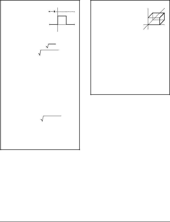
INFINITE SQUARE-WELL POTENTIAL or "Particle in a Box"
This is a concept that applies to many physical situations. Consider a two-dimensional box in which a particle may be trapped by an infinite voltage potential on either side. The problem is an application of the
Schrödinger Wave Equation.
V(x)
x
0 L
The particle may have various energies represented by waves that must have an amplitude of zero at each boundary 0 and L. Thus, the energies are quantized. The probability of the particle's location is also expressed by a wave function with zero values at the boundaries.
|
|
|
|
|
|
|
|
æ npx ö |
|
||
Wave function: |
yn |
( x) = A sin ç |
|
÷ |
|
||||||
L |
|
||||||||||
|
|
|
|
è |
ø |
|
|||||
Energy levels: |
En |
= n2 |
|
p2h2 |
|
|
|
|
|||
|
2mL2 |
|
|
|
|||||||
|
|
|
|
|
|
|
|
|
|
||
Probability of a particle being |
|
x2 |
|
||||||||
found between x1 and x2: |
P = òx= x1 |
Y *Y dx |
|||||||||
A = |
2 |
normalization constant |
|
|
|
||||||
|
L |
|
|
|
|
|
|
|
|
|
|
a useful identity: |
sin2 θ = |
1 |
(1 − cos 2θ) |
|
|
||||||
|
|
|
|||||||||
|
|
|
|
2 |
|
|
|
|
|
|
|
Tom Penick tomzap@eden.com www.teicontrols.com/notes 12/12/1999 Page 12 of 22
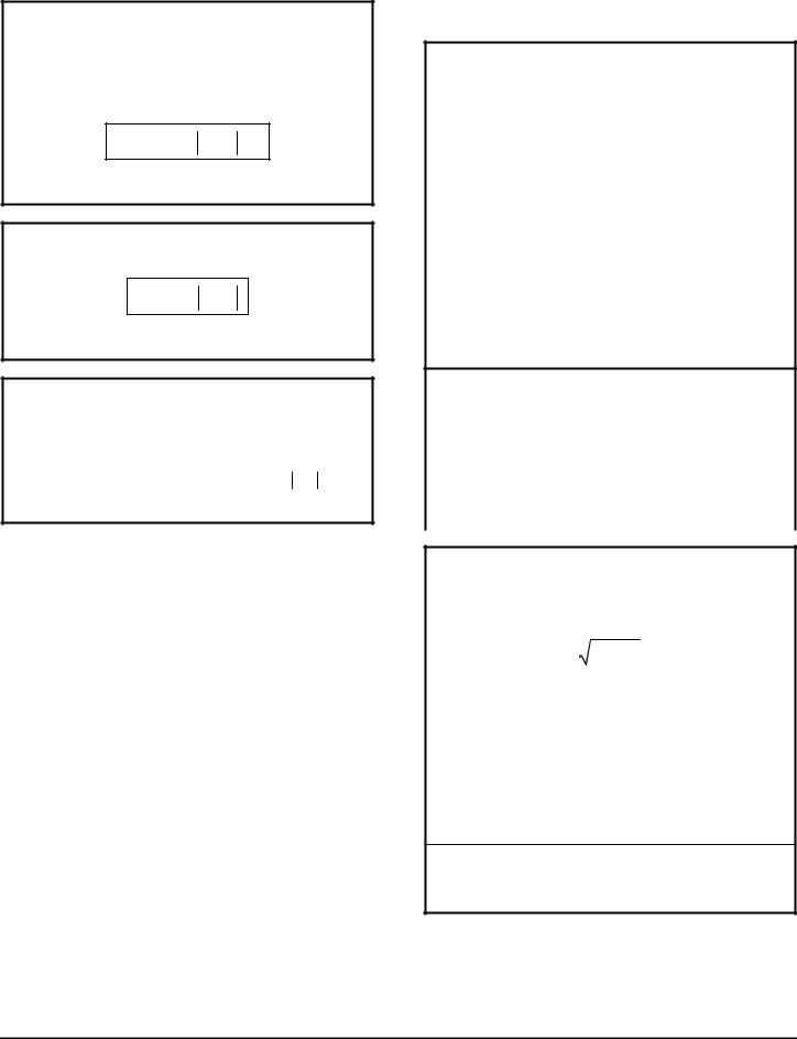
POTENTIAL BARRIER
When a particle of energy E encounters a barrier of potential V0, there is a possibility of either a reflected wave or a transmitted wave.
|
V(x) |
|
|
particle |
|
|
|
V0 |
|
|
|
|
0 |
|
x |
|
L |
||
Region I |
Region II |
Region III |
|
for E > V0: |
|
|
|
|
|
|
|
kinetic energy: |
K = E -V0 |
|
|
|
|
||
wave number: |
kI |
= kIII = |
2mE / h |
|
|
|
|
|
kII = 2m ( E -V0 ) / h |
|
|
|
|||
incident wave: |
jI |
= AeikI x |
|
|
|
|
|
reflected wave: jI |
= Be−ikI x |
|
|
|
|
||
transmitted wave: |
jIII = FekI x |
|
|
|
|||
|
|
æ |
V 2 sin2 (k |
II |
L) ö−1 |
||
trans. probability: |
T = ç1+ |
0 |
|
÷ |
|||
4E (E -V ) |
|||||||
|
|
ç |
÷ |
||||
|
|
è |
|
0 |
ø |
||
reflection probability: R =1-T
for E < V0: Classically, it is not possible for a particle of energy E to cross a greater potential V0, but there is a quantum mechanical possibility for this to happen called tunneling.
kinetic energy: K =V0 - E |
|
|
||
wave #, region II: |
k = 2m (V0 - E ) / h |
|
||
|
|
|
||
|
æ |
V 2 sinh2 (kL) ö−1 |
||
trans. probability: |
T = ç1+ |
0 |
÷ |
|
4E (V - E ) |
||||
|
ç |
÷ |
||
|
è |
0 |
ø |
|
when kL ?1: T =16 |
E æ |
|
|
E ö |
|
||
|
ç1 |
- |
|
|
÷e−2 |
κL |
|
|
|
|
|||||
|
V0 è |
|
V0 ø |
|
|||
3D INFINITE POTENTIAL BOX
Consider a three-dimensional box with zero voltage potential inside the box and infinite voltage outside. A particle trapped in the box is described by a wave function and has quantized energy levels.
z |
y |
|
|
L3 |
|
|
L2 |
0 |
x |
L1 |
Time-independent Schrödinger Wave Equation in three dimensions:
2 |
æ |
2 |
y |
2 |
y |
2 |
y |
ö |
|
|||
- |
h |
ç |
¶ |
+ |
¶ |
+ |
¶ |
÷ |
+V y = Ey |
|||
|
|
2 |
|
2 |
|
2 |
||||||
|
2m è |
¶x |
|
¶y |
|
¶z |
ø |
|
||||
Wave equation for the 3D infinite potential box:
|
|
|
æ n p x ö |
æ n p y ö |
æ n p z ö |
|||||||||||||||||
|
yn1 n2 n3 |
= Asin ç |
1 |
|
|
÷sin |
ç |
|
2 |
|
|
÷sin ç |
|
3 |
|
|
÷ |
|||||
|
|
|
|
|
|
|
|
|
|
|
||||||||||||
|
|
è |
L1 ø |
è |
|
L2 ø |
è |
|
L3 ø |
|||||||||||||
|
|
|
|
|
|
|
|
|
|
|
|
|
|
|
|
|||||||
|
|
|
En1 n2 n3 |
= |
|
p2h2 æ n12 |
+ |
|
n22 |
+ |
n32 ö |
|
||||||||||
Energy levels: |
|
|
|
ç |
|
|
|
|
÷ |
|
|
|||||||||||
|
2m |
|
2 |
2 |
2 |
|
||||||||||||||||
|
|
|
|
|
|
|
|
è |
L1 |
|
|
|
L2 |
|
L3 |
ø |
|
|
||||
Degenerate energy levels may exist—that is, different combinations of n-values may produce equal energy values.
Tom Penick tomzap@eden.com www.teicontrols.com/notes 12/12/1999 Page 13 of 22

SCHRÖDINGER'S EQUATION – 3D
SPHERICAL spherical coordinate form:
|
1 ¶ æ 2 |
¶yö |
|
1 ¶ æ |
¶yö |
|
1 ¶2y |
|
2m |
|||||||||||||
|
|
|
|
çr |
|
÷+ |
|
|
|
|
çsinq |
|
÷+ |
|
|
|
|
|
|
+ |
|
(E-V)y=0 |
|
2 |
|
|
2 |
|
|
|
2 |
2 |
2 |
|
2 |
||||||||||
|
r |
|
¶r è |
¶r ø |
r |
sinq¶qè |
¶qø |
r |
sin |
q ¶q |
|
h |
||||||||||
separation of variables using: |
Ψ (r,θ,φ) = R (r) f (θ) g (φ) |
|||||||||||||||||||||
We can obtain a form with terms of g on one side and terms of R and f on the other. These are set equal to the constant ml2. ml turns out to be an integer.
Another seperation is performed for R and f and the constant is l(l+1), where l is an integer. The three equations are:
Azimuthal equation:
|
1 d 2 g |
+ m |
2 |
= |
0 |
|
Þ g = Ae |
im φ |
|
|
|
|
|
||||||||||||||||
|
|
|
|
|
|
|
|
|
|
|
|
|
l |
|
|
|
|
|
|||||||||||
|
g df2 |
|
|
|
|
|
|
|
|||||||||||||||||||||
|
|
|
l |
|
|
|
|
|
|
|
|
|
|
|
|
|
|
|
|
||||||||||
Radial equation: |
|
|
|
|
|
|
l (l +1) |
|
|||||||||||||||||||||
|
1 d æ |
|
2 dR ö |
|
|
2m |
(E -V ) R - |
|
|||||||||||||||||||||
|
|
|
|
|
|
|
|
ç r |
|
|
|
|
÷ |
+ |
|
|
|
|
|
|
R = 0 |
||||||||
|
r |
2 |
|
|
|
|
|
|
|
|
|
|
2 |
|
r |
2 |
|
||||||||||||
|
|
|
|
|
dr è |
|
|
dr ø |
|
|
h |
|
|
|
|
|
|
|
|
||||||||||
Angular Equation: |
|
|
|
|
|
|
|
|
|
|
|||||||||||||||||||
|
|
1 |
|
|
|
d æ |
|
|
|
|
df ö |
|
é |
|
|
m 2 |
ù |
|
|
||||||||||
|
|
|
|
|
|
|
|
|
|
|
|
çsin q |
|
|
|
÷ |
+ êl (l +1) - |
|
l |
|
ú f |
= 0 |
|||||||
|
sin q dq |
|
dq |
|
2 |
|
|||||||||||||||||||||||
|
è |
|
|
|
|
|
ø |
|
ë |
|
sin |
q û |
|
||||||||||||||||
ml = magnetic quantum number; integers ranging from –l to +l
l = orbital angular momentum quantum number h = Planck's constant divided by 2p [J-s]
E = energy
V = voltage; can be a function of space and time (x,t) m = mass [kg]
NORMALIZING WAVE FUNCTIONS
To normalize a function, multiply the function by its complex conjugate and by the square of the normalization constant A. Integrate the result from -¥ to ¥ and set equal to 1 to find the value of A. The normalized function is the original function multiplied by A.
To normalize the wave function Ψ(x):
ò−∞∞ |
2 |
AY dx ® A2 ò−∞∞ Y2dx |
Where Ψ is an even function, we can simplify to:
∞ ∞
2A2 ò0 Y2dx and find A: 2A2 ò0 Y2dx =1
Some relations for definite integrals will be useful in solving this equation; see CalculusSummary.pdf page 3.
To normalize the wave function Ψ(r), where r is the radius in spherical coordinates:
∞ 2 ∞
ò0 r 2 AY dr ® A2 ò0 r 2 Y2dr =1
Note that we integrate from 0 to ∞ since r has no negative values.
To normalize the wave function Ψ(r,θ,φ):
A2 ò0∞ dr r 2 AY 2 ò0π dq sin q ò02π df = 1
Note that dr, dθ, and dφ are moved to the front of their respective integrals for clarity.
Rnl(r) RADIAL WAVE FUNCTIONS
for the hydrogen atom
n |
l |
|
|
|
|
|
|
|
|
|
|
|
|
|
|
|
|
|
|
|
Rnl(r) |
|
|
|
|
|
|
|||||
1 |
0 |
2 |
|
|
|
e |
− r / a0 |
|
|
|
|
|
|
|
|
|
|
|
|
|
|
|
|
|
|
|
||||||
|
a03 / 2 |
|
|
|
|
|
|
|
|
|
|
|
|
|
|
|
|
|
|
|
|
|
|
|
|
|
||||||
|
|
|
|
|
|
|
|
|
|
|
|
|
|
|
|
|
|
|
|
|
|
|
|
|
|
|
|
|
||||
|
|
æ |
|
- |
|
r |
|
ö |
|
e |
−r / 2 a0 |
|
|
|
|
|
|
|
|
|
|
|
|
|||||||||
|
|
|
|
|
|
|
|
|
|
|
|
|
|
|
|
|
|
|
|
|
|
|
|
|||||||||
2 |
0 |
ç w |
|
|
|
|
|
÷ |
|
|
|
|
|
|
|
|
|
|
|
|
|
|
|
|
|
|
|
|
||||
|
|
|
|
|
|
|
|
|
|
3 / 2 |
|
|
|
|
|
|
|
|
|
|
|
|
|
|||||||||
|
|
è |
|
|
|
|
a0 ø (2a0 ) |
|
|
|
|
|
|
|
|
|
|
|
|
|||||||||||||
|
|
|
r |
|
|
|
e |
−r / 2a0 |
|
|
|
|
|
|
|
|
|
|
|
|
|
|
|
|
|
|
||||||
2 |
1 |
|
|
|
|
|
|
|
|
|
|
|
|
|
|
|
|
|
|
|
|
|
|
|
|
|
|
|
||||
|
|
|
|
|
|
|
|
|
|
|
|
|
|
|
|
|
|
|
|
|
|
|
|
|
|
|
|
|
|
|
||
|
a0 |
|
|
3 ( |
2a |
)3 / 2 |
|
|
|
|
|
|
|
|
|
|
|
|
|
|
|
|
||||||||||
|
|
|
|
|
|
|
|
|
|
|
|
|
|
|
|
|
|
|
|
|
||||||||||||
|
|
|
|
|
|
|
|
|
|
|
0 |
|
|
|
|
|
|
|
|
|
|
|
|
|
|
|
|
|
|
|||
3 |
0 |
1 |
3 / 2 |
|
2 æ |
27 -18 |
|
r |
+ |
2 |
r 2 |
ö |
− r / 3 a |
|||||||||||||||||||
|
|
|
|
|
|
|
|
|
|
ç |
|
|
|
|
2 |
÷e |
0 |
|||||||||||||||
|
|
|
(a |
) |
|
|
|
|
|
81 |
3 |
è |
|
|
|
|
|
|
a0 |
|
|
a |
0 |
ø |
|
|||||||
|
|
0 |
|
|
|
|
|
|
|
|
|
|
|
|
|
|
|
|
|
|
|
|
|
|
|
|
||||||
|
|
1 |
|
|
|
|
|
4 æ |
6 - |
r ö r |
e |
− r / 3a0 |
|
|
||||||||||||||||||
3 |
1 |
|
|
|
|
|
|
|
|
|
|
|
ç |
|
|
÷ |
|
|
|
|
|
|
|
|||||||||
|
(a0 ) |
3 / 2 |
|
81 6 |
|
|
|
|
|
|
|
|
|
|||||||||||||||||||
|
|
|
|
|
|
|
|
è |
|
|
|
a0 ø a0 |
|
|
|
|
|
|
||||||||||||||
3 |
2 |
1 |
|
|
|
|
|
|
|
|
4 |
|
|
|
|
r 2 |
e |
−r / 3a |
|
|
|
|
|
|
||||||||
|
|
|
|
|
|
|
|
|
|
|
|
|
|
|
|
|
|
|
0 |
|
|
|
|
|
|
|
||||||
|
|
|
(a |
)3 / 2 |
|
81 |
30 a 2 |
|
|
|
|
|
|
|
|
|
|
|
|
|||||||||||||
|
|
0 |
|
|
|
|
|
|
|
|
|
|
|
|
|
0 |
|
|
|
|
|
|
|
|
|
|
|
|
|
|||
a0 = Bohr radius 5.29177×10⁻¹¹ m
Tom Penick tomzap@eden.com www.teicontrols.com/notes 12/12/1999 Page 14 of 22
P(r)dr RADIAL PROBABILITY
The radial probability is a value from 0 to 1 indicating the probability of a particle occupying a certain area radially distant from the center of orbit. The value is found by integrating the right-hand side of the expression over the interval in question:
P(r) dr = r 2 R (r ) 2 dr
r = orbit radius
R(r) = radial wave function, normalized to unity
P(r) RADIAL PROBABILITY DENSITY
The radial probability density depends only on n and l.
P(r) = r 2 R (r ) 2
r = orbit radius
R(r) = radial wave function, normalized to unity
árñ RADIAL EXPECTATION VALUE average radius (radial wave function):
 r
r = òr∞=0 r P (r )dr = òr∞=0 r3 R(r ) dr
P(r) = probability distribution function P (r ) = r2 R (r ) 2 dr
R(r) = radial wave function, normalized to unity
ATOMS
QUANTUM NUMBERS
n= principal quantum number, shell number, may have values of 1, 2, 3, …
l = orbital angular momentum quantum number, subshell number, may have values of 0 to n-1. These values are sometimes expressed as letters: s=0, p=1, d=2, f=3, g=4, h=5, …
ml = magnetic quantum number, may have integer values from -l to +l for each l. (p251)
ms = magnetic spin quantum number, may have values of +½or -½
Then we introduce these new ones: s = intrinsic quantum number, s =1/2 (p238)
j = total angular momentum quantum number, j = l ± s, but j is not less than 0. (p257)
mj = magnetic angular momentum quantum number, may have values from -j to +j (p257)
Example, for n = 3:
l = |
|
0 |
|
1 |
|
|
|
2 |
|
|
|
||
j = |
|
1/2 |
1/2 |
|
|
3/2 |
|
3/2 |
|
|
5/2 |
|
|
mj |
= |
-1/2 +1/2 |
-1/2 +1/2 |
-3/2 -1/2 |
-3/2 -1/2 +1/2 +3/2 |
|
-5/2 -3/2 -1/2 |
||||||
|
|
|
+1/2 +3/2 |
|
|
|
|
+1/2 +3/2 +5/2 |
|||||
|
|
|
|
|
|
|
|
|
|||||
|
|
|
|
|
|
|
|
|
|
|
|
|
|
ml = |
0 |
-1 |
0 |
+1 |
-2 |
-1 |
0 |
|
+1 |
+2 |
|||
ms |
= |
-1/2 |
-1/2 |
-1/2 |
-1/2 |
-1/2 |
-1/2 |
-1/2 |
|
-1/2 |
-1/2 |
||
+1/2 |
+1/2 |
+1/2 |
+1/2 |
+1/2 |
+1/2 |
+1/2 |
|
+1/2 |
+1/2 |
||||
|
|
|
|||||||||||
L ORBITAL ANGULAR MOMENTUM
Classically, orbital angular momentum is ρr or mvr. The orbital angular momentum L is a vector quantity. It components are as follows:
Magnitude: |
L = h l (l +1) |
Z-axis value: |
Lz = ml h |
The values of Lx and Ly cannot be determined exactly but obey the following relation:
L2 = L2x + L2y + L2z
h = Planck's constant divided by 2π [J-s]
l = orbital angular momentum quantum number
ml = magnetic quantum number; integers ranging from –l to +l
The orbital angular momentum quantum |
l = 0 1 2 3 4 5 |
|
number was originally given letter values |
||
s p d f g h |
||
resulting from early visual observations: |
||
|
||
sharp, principal, diffuse, fundamental |
|
Tom Penick tomzap@eden.com www.teicontrols.com/notes 12/12/1999 Page 15 of 22

S SPIN ANGULAR MOMENTUM
The spin angular momentum is (insert some illuminating explanation here).
Magnitude: |
|
z |
S = h s (s +1) = h 3 / 4 |
|
1 |
+ |
2 h |
|
z component: |
|
S= h 3/4 |
|
|
|
Sz = ms h = ±h / 2 |
|
1 |
|
- |
2 h |
J TOTAL ANGULAR MOMENTUM
The vector sum of the orbital angular momentum and the spin angular momentum. This applies to 1- electron and many-electron atoms.
J = L + S
J (the magnitude?) is an integer value from |L-S| to L+S.
ALLOWED TRANSITIONS
The allowed energy level transitions for 1-electron atoms are
n: any |
l: ±1 |
mj: 0, ±1 |
j: 0, ±1 |
ZEEMAN SPLITTING ("ZAY· mahn")
When a single-electron atom is under the influence of an external magnetic field (taken to be in the z-axis direction), each energy level (n=1,2,3,…) is split into multiple levels, one for each quantum number ml. The difference in energy is:
E = μB Bml
E = difference in energy between two energy levels [J]
μB = Bohr magneton 9.274078×10⁻²⁴ J/T B = magnetic field [T]
ml = magnetic quantum number; integers ranging from –l to +l
μ MAGNETIC MOMENT
Both the magnetic moment μ and the orbital angular momentum L are vectors:
ì = − e L
2m
m = mass of the orbiting particle [kg]
MANY-ELECTRON ATOMS
SPECTROSCOPIC SYMBOLS
The energy state of an atom having 1 or 2 electrons in its outer shell can be represented in the form
n2S +1Lj
n = shell number
S = intrinsic spin angular momentum quantum number; ½ for a single-electron shell, 0 or 1 (S1 + S2) for the 2- electron shell
L = angular momentum quantum number; l for singleelectron shell, L1 + L2 for a 2-electron shell, expressed as a capital letter: S=0, P=1, D=2, F=3, G=4, H=5, I=6.
j = total angular momentum quantum number j = l ± s. I'm not sure how to tell whether it's plus or minus, but I think it has to be the lower value of j to be in the ground state. j is positive only.
ORDER OF ELECTRON FILLING
Here's a way to remember the order in which the outer shells of atoms are filled by electrons:
Form groups of l-numbers like this. The first |
s |
|
p s |
||
group is just the lowest value for l: s. The next |
||
d p s |
||
value of l is p; form a new group of p with s. |
||
The third value of l is d; form the third group |
f d p s |
|
with d, p, and s. You get a list of groups like |
g f d p s |
|
this: |
h g f d p s |
|
Now, in a column, write each group twice |
1s |
|
beginning with the single s that is the first |
2s |
|
group. |
p |
|
Next number each s beginning with 1, placing |
3s |
|
the number in front of the s. This is as far as |
p |
|
I have gone with the list at right. |
4s |
|
The next step is to number each p beginning |
d |
|
p |
||
with the number 2. |
||
Then number each d beginning with the |
5s |
|
f |
||
number 3. |
||
d |
||
Number each f beginning with 4, and so on. |
||
p |
||
The result will be the order of filling (there are |
6s |
|
a few exceptions) and will look like this: |
f |
|
1s 2s 2p 3s 3p 4s 3d 4p 5s 4d 5p 6s 4f 5d |
d |
|
p |
||
and so on. |
||
7s |
||
|
||
|
and so on. |
Tom Penick tomzap@eden.com www.teicontrols.com/notes 12/12/1999 Page 16 of 22

g LANDÉ g FACTOR
A dimensionless number that helps make physics complicated. Used in ANOMALOUS ZEEMAN SPLITTING
g = 1+ J ( J +1) + S (S +1) − L (L +1)
2J ( J +1)
ALLOWED PHOTON TRANSITIONS
The allowed photon energy level transitions for manyelectron atoms are
L: |
±1 |
J: 0, ±1, |
but J can't transition from 0 to 0. |
S: |
0 |
mj: 0, ±1, |
but can't transition from 0 to 0 |
|
|
|
when J=0. |
Other transitions are possible—just not likely.
θ MINIMUM ANGLE BETWEEN J AND
THE Z-AXIS
There were exercises where we had to calculate this. I don't know what the significance is. This is done similarly for L and S as well.
Example: j = 5
|
|
|
|
j ´ h |
2 |
|
cos q = |
|
|
|
|
→ |
|
h |
|
j ( j +1) |
||||
|
|
|||||
cos2 q = |
|
|
j2 |
→ cos2 θ = |
||
j |
( |
j +1 |
||||
|
|
|
) |
|
|
|
cos θ =
j
j +1
|
|
|
z |
|
|
|
+ 25 h |
θ |
J = h j(j+1) |
||
|
+ 23 h |
|
|
||
j |
+ |
21 |
h |
|
|
- |
21 |
h |
|
|
|
( j +1) |
|
|
|||
|
- |
23 |
h |
|
|
|
- |
25 |
h |
|
|
SPLITTING DUE TO SPIN
For each state described by quantum numbers n, l, ml, there are two states defined by the magnetic spin numbers
ms = ±1/2. These two levels have the same energy except when the atom is influenced by an external magnetic field.
z
1
+ 2 h


S = h 3/4
3/4
- 12 h
The lower of the two energy levels is aligned with the magnetic field.
E= hc Δλ
λ2
E = difference in energy between two (split) energy levels ms = ±1/2 [J]
Δλ = difference in wavelengths for the transitions to the ground state for each energy level [m]
λ = wavelength for the transitions to the ground state for the lower of the two energy levels (the greater of the two wavelengths) [m]
h = Planck's constant 6.6260755×10⁻³⁴ J-s c = speed of light 2.998 × 10⁸ m/s
SPIN-ORBIT ENERGY SPLITTING
Spin-orbit energy splitting is the splitting of energy levels caused by an internal magnetic field due to spin. This produces a greater E than the spin splitting described above. p265
P.E. due to spin V = −ì s ·B
z-component |
mz |
= -gs |
æ |
eh ö J z |
|
|
|||
|
ç |
|
÷ |
|
|
|
|
||
|
|
|
|
|
|||||
|
|
|
è |
2me ø h |
|
|
|||
energy level difference |
|
E = gs |
eh |
B |
|||||
|
|
||||||||
|
|
|
|
|
|
|
|
m |
|
|
|
|
|
|
|
|
|
e |
|
e = q = electron charge 1.6022×10⁻¹⁹ C
h = Planck's constant divided by 2π [J-s]
jz = z-component of the total angular momentum
E = difference in energy between two (split) energy levels ms = ±1/2 [J]
gs = 2, the gyromagnetic ratio
me = mass of an electron 9.1093897×10⁻³¹ kg B = internal magnetic field [T]
Tom Penick tomzap@eden.com www.teicontrols.com/notes 12/12/1999 Page 17 of 22

ANOMALOUS ZEEMAN SPLITTING
("ZAY· mahn")
In addition to the Zeeman splitting of the ml energy levels described previously, and the spin-orbit energy splitting described above, there is a splitting of the mj levels when an external magnetic field is present. The difference in energy between levels is:
V = mB Bext gmj
V = difference in energy between two energy levels [J]
μB = Bohr magneton 9.274078×10⁻²⁴ J/T Bext = external magnetic field [T]
g = Landé factor [no units]
mj = magnetic angular momentum quantum number; halfintegers ranging from –j to +j
STATISTICAL PHYSICS
v*, v , vrms MOLECULAR SPEEDS [m/s]
Maxwell speed |
|
|
|
|
|
|
|
|
|
|
|
|
|
|
− |
1 |
βmv2 |
||||||||
distribution: |
|
F (v) dv = 4pCe 2 |
|
|
|
v2 dv |
|||||||||||||||||||
|
|
|
|
|
|
|
|
|
|
|
|
|
|
|
|
|
|
|
|
|
|||||
v* most probable |
v* = |
|
2 |
|
|
|
= |
|
|
2kT |
|
|
|
|
|||||||||||
speed: |
|
bm |
|
|
|
m |
|
|
|
|
|
||||||||||||||
|
|
|
|
|
|
|
|
|
|
|
|
|
|
||||||||||||
|
|
|
|
|
|
|
|
|
|
|
|
|
|
|
|
|
|
|
|
|
|
||||
|
|
|
|
|
|
|
|
|
|
|
|
|
|
|
|
|
|
|
|
|
|||||
|
|
|
mean speed: |
|
|
= |
4 |
|
|
|
|
|
kT |
|
|
|
|
|
|
|
|
||||
v |
|
|
|
|
|
|
|||||||||||||||||||
|
|
v |
|
|
|
|
|
|
|||||||||||||||||
|
|
|
2p |
|
m |
|
|
|
|
|
|
|
|
|
|
|
|||||||||
|
|
|
|
|
|
|
|
|
|
|
|
|
|
|
|
|
|
|
|||||||
|
|
|
|
|
|
|
|
|
|
||||||||||||||||
vrms |
root mean |
|
|
|
= é |
|
|
ù1 / 2 |
= |
3kT |
|
|
|||||||||||||
v |
v2 |
||||||||||||||||||||||||
square speed: |
|
rms |
ë û |
|
|
|
|
|
|
|
|
m |
|
||||||||||||
v = velocity [m/s]
C = normalization constant
k = Boltzmann's constant 1.380658×10⁻²³ J/K T = temperature [K]
m = mass of the molecule [kg]
β = the parameter 1/kT [J-1]
ENERGY DISTRIBUTION
Derived from Maxwell's speed distribution:
F (E ) = 8pC e−βE E1 / 2
2m3 / 2
FMB MAXWELL-BOLTZMANN FACTOR
The Maxwell-Boltzmann factor is a value between 0 and 1 representing the probability that an energy level E is occupied by an electron (at temperature T). This is for classical systems, such as ideal gases. One way to determine if Maxwell-Boltzmann statistics are valid is to compare the de Broglie wavelength λ = h/p of a typical particle with the average interparticle spacing d. If λ<<d then Maxwell-Boltzmann statistics are generally acceptable.
|
æ V ö1 / 3 |
|||
F = Ae−βE |
||||
d = ç |
|
÷ |
||
|
||||
MB |
è |
N ø |
||
|
||||
A = normalization constant
β = the parameter 1/kT [J-1] d = space between atoms [m]
N = number of particles in volume V. Note that
Avogadro's number, 6.022×10²³, is the number of gas molecules in 22.4 liters, or 22.4×10⁻³ m3, at 0°C and 1 atmosphere. Also, gas volume is proportional to temperature: V1/T1=V2/T2.
Tom Penick tomzap@eden.com www.teicontrols.com/notes 12/12/1999 Page 18 of 22
FFD FERMI-DIRAC DISTRIBUTION
A value between 0 and 1 indicating the probability than an energy state is occupied by an electron. The Fermi-Dirac distribution is valid for fermions, particles with half-integer spins that obey the Pauli principle. Atoms and molecules consisting of an even number of fermions must be considered bosons when taken as a whole because their total spin will be zero or an integer.
1
FFD = B1ebE +1
B1 = normalization constant
β = the parameter 1/kT [J-1]
FBE BOSE-EINSTEIN DISTRIBUTION
The Bose-Einstein distribution is valid for bosons, particles with zero or integer spins that do no obey the Pauli principle. Photons, pions, and liquid 4He are bosons.
1
FBE = B2ebE -1
B2 = normalization constant
β = the parameter 1/kT [J-1]
EF FERMI ENERGY [eV]
The Fermi energy depends on the density of electrons in the material. The Fermi-Dirac distribution is modified to include the Fermi energy:
FFD = |
|
1 |
|
|
|
|
|
|
|
éb |
E -E |
ù |
|
|
|
eë ( |
|
F )û +1 |
|
The relationship between the Fermi energy and the number density of particles is:
h2 æ 3N ö2 / 3
EF = 8m çè pL3 ÷ø
FFD = Fermi-Dirac distribution, a value from 0 to 1 indicating the probability that an energy state is occupied
β = the parameter 1/kT [J-1]
h = Planck's constant 6.6260755×10⁻³⁴ J-s m = mass of the particle [kg]
N/L3 = number density of the particles [m-3]
TF FERMI TEMPERATURE
The Fermi temperature may be quite high, 80,000 K for copper.
TF = EF k
EF = Fermi Energy [eV]
k = Boltzmann's constant 1.380658×10⁻²³ J/K
uF |
FERMI SPEED |
|
||||||
|
|
|
|
|
|
|
|
|
The Fermi speed, |
uF = |
2EF |
|
|
|
|
|
|
m |
|
|
|
|
|
|
||
|
|
|
|
|
|
|
|
|
comes from the definition: EF |
= |
1 |
muF |
2 |
||||
|
|
|||||||
|
|
|
2 |
|
|
|||
EF = Fermi Energy [eV]
m = mass (probably of the electron) [kg]
ENERGY STATES IN "PHASE SPACE"
The points in the 1/8 sphere represent the energy states of a particle in a cube, see 3D INFINITE POTENTIAL BOX p13.
Energy level at radius r
E = r 2 E1
where E1 = h2 / 8mL2
(a constant equal to 1/3 of the ground state energy)
and r = n 2 |
+ n 2 |
+ n 2 |
|
1 |
2 |
3 |
|
and E is whatever energy |
|
||
the problem is concerned |
n1 |
||
with. |
|
|
|
n3 |
integer |
|
|||
spacing |
energy |
||||
|
|
|
|||
|
|
|
|
states |
|
3 |
|
|
|
energy |
|
|
|
|
levels |
||
2 |
|
|
|
|
|
1 |
|
|
|
n2 |
|
1 |
1 |
2 |
3 |
||
Dr |
|||||
r |
|
|
|||
2 |
|
|
|||
 3
3
Nr Number of energy states in a sphere of radius r, i.e. the number of energy states there are with energy less than E:
|
|
|
|
|
|
|
|
p æ E ö3 / 2 |
||||||
Nr |
= 2 |
æ 1 öæ 4 |
pr |
3 |
ö |
|
Nr = |
|||||||
ç |
|
֍ |
|
|
÷ |
or |
|
ç |
|
÷ |
||||
8 |
3 |
|
3 |
|
||||||||||
|
|
è |
øè |
|
|
ø |
|
|
è |
E1 ø |
||||
|
|
|
|
|
|
|
|
|
|
|
|
|
|
|
where the factor of 2 is due to spin degeneracy, and the factor of 1/8 is because the energy states only occupy 1/8 of the sphere where n1, n2, n3 are all positive.
g(E) DENSITY OF ENERGY STATES
Number of states per unit energy
g ( E ) = |
p |
-3 / 2 |
|
1/ 2 |
g ( E ) = |
DN |
|
= |
dN |
|
|
E1 |
E |
|
|
r |
|
r |
|||
2 |
|
|
|
dE |
||||||
|
|
|
|
|
DE |
|||||
Nr = number of energy states in a sphere of radius r E1 = a constant equal to 1/3 of the ground state energy
Tom Penick tomzap@eden.com www.teicontrols.com/notes 12/12/1999 Page 19 of 22

n(E) DENSITY OF OCCUPIED STATES
Number of occupied states per unit energy
n ( E) = FFD × g ( E)
ìg (E ), for E < E at T=0, n ( E ) = í F
î0, for E > EF
FFD = Fermi-Dirac distribution, a value from 0 to 1 indicating the probability that an energy state is occupied
Tom Penick tomzap@eden.com www.teicontrols.com/notes 12/12/1999 Page 20 of 22