4.3.5 Summary of 3d Graphics
Three-dimensional plots (or 3D graphs) can be created by this numerical software.
Matlab provides many facilities for visualization of 3D information or data (x, y, z). The facilities include built-in functions for plotting wire-frame objects, space-curves, shaded surfaces.
Also, automatic generation of contours, volumetric data display, light sources, interpolation of colors and displaying externally-created images.
Typing ‘help graph3d’ in the command window gives a list of functions available for general 3D graphs.
This is a kind of ‘catalog’ of the most popular 3D graphics functions.
You can use these instructions for your needs simply by following the examples. The ‘meshgrid’ function must be first understood.
Examples:
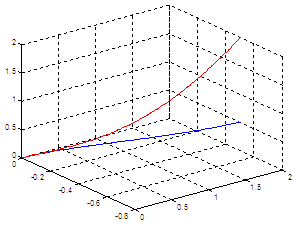
plot3
|
t = 0 : .01 : 1; x = 2*t; y = -0.5*t.^2; z1 = t.^3/2; z2 = t.^3/.5; plot3(x,y,z1,'b', x,y,z2,'r') grid
|
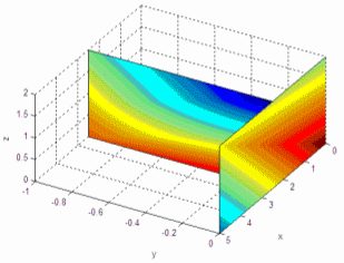
fill3 |
x = [0 2.5; 5 2.5; 5 2.5; 0 2.5]; y = [0 0; 0 -1; 0 -1; 0 0]; z = [0 0; 0 0; 2 2; 2 2]; fill3(x,y,z, rand(4,2)) xlabel('x'); ylabel('y'); zlabel('z'); view(120, 50) grid
|
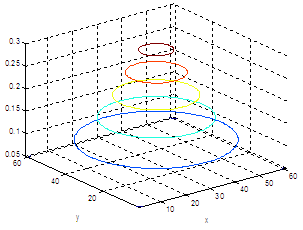
contour3
|
X = -3:.1:3; [x,y] = meshgrid(X,X); z = 1./(3+x.^2+y.^2); contour3(z) xlabel('x'); ylabel('y');
|
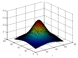
surf
|
X = -3 : .1 : 3; [x,y] = meshgrid(X,X); z = 1./(3+x.^2+y.^2); surf(z) xlabel('x'); ylabel('y');
|
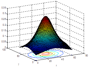
surfc
|
X = -3 : .1 : 3; [x,y] = meshgrid(X,X); z = 1./(3+x.^2+y.^2); surfc(z) view(-30,20) xlabel('x'); ylabel('y');
|
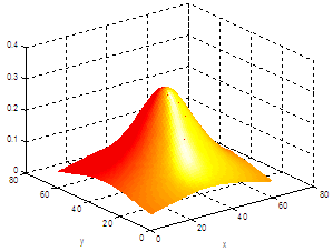
surfl |
X = -3 : .1 : 3; [x,y] = meshgrid(X,X); z = 1./(3+x.^2+y.^2); surfl(z) shading interp colormap hot xlabel('x'); ylabel('y');
|
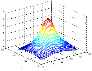
mesh |
X = -2 : .1 : 2; [x,y] = meshgrid(X,X); z = 5./(1+x.^2+y.^2); mesh(z) xlabel('x'); ylabel('y');
|
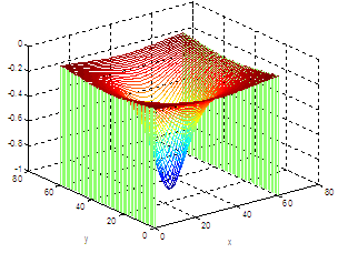
waterfall |
X = -3 : .1 : 3; [x,y] = meshgrid(X,X); z = -1./(1+x.^2+y.^2); waterfall(z) hidden off xlabel('x'); ylabel('y');
|
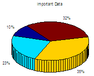
pie3 |
data = [10 23 35 32];
pie3(data)
title('Important Data')
|
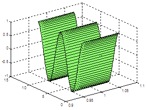
ribbon |
x = 0 : .1 : 4*pi;
y = cos(x);
ribbon(x,y,.1)
|
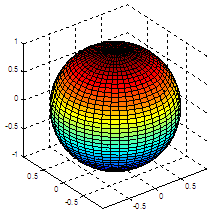
sphere |
sphere(45) axis 'equal'
|
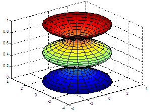
cylinder |
z = 0: .03 : 1; r = cos(4*pi*z)+2; cylinder(r)
|
Individual tasks
1 |
|
2 |
|
3 |
|
4 |
|
5 |
|
6 |
|
7 |
|
8 |
|
9 |
|
10 |
|
11 |
|
12 |
|
13 |
|
14 |
|
15 |
|
16 |
|
17 |
|
18 |
|
19 |
|
20 |
|
21 |
, -2.1 ≤ x ≤ 2.1 and -6 ≤ y ≤ 6 |
22 |
|