4.3.3 Instructions: sphere, plot3, mesh

The function 'sphere'

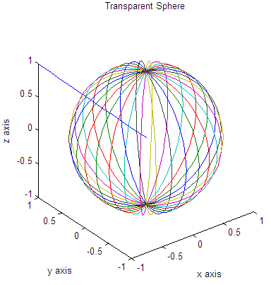
In this part, we demonstrate the use of the function 'sphere'. We are going to draw a unit sphere centered at the origin and generated by matrices x, y and z, of size 31 x 31 each.

Just as an exercise, we also add a line going from the center of the sphere to one of the corners in the figure (within the 3D plot). This is important to note the fact that we can add several shapes to the figure, by using the instruction ' hold on '.

Example:

We plot a transparent sphere using appropriate commands. We add a line from the center of the sphere to one corner of the containing box. We demonstrate the use of the instruction 'axis' with the parameter 'square'.

% cleans the workspace

clc; clear; close all

% returns the coordinates of a sphere in three

% matrices that are (n+1)-by-(n+1) in size

[x, y, z] = sphere(30);

plot3(x,y,z)

% keeps the proportions in place and writes appropriate info.

axis('square')

title('Transparent Sphere')

xlabel('x axis')

ylabel('y axis')

zlabel('z axis')

% keeps the above sphere in order to superimpose a line

hold on

% the line goes from (-1, 1, 1) to (0, 0, 0)

a = -1 : .1 : 0;

b = 1 : -.1 : 0;

c = b;

plot3(a, b, c)

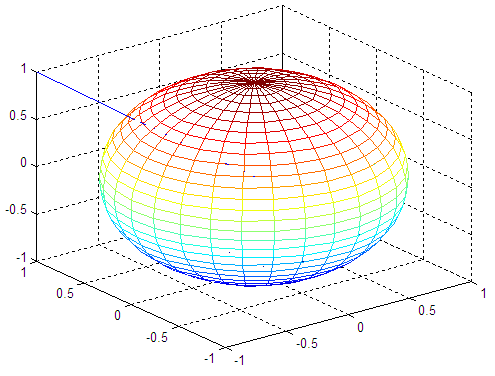
% draws the sphere in another format and in another figure

% see what happens if we don't use the axis('square') instruction

figure

mesh(x,y,z)

hold on

plot3(a, b, c)

And the resulting figures are:

Examples

In this example we make a summarization of the use of the following 3D plot instructions:

• meshgrid;

• figure;

• contour3;

• mesh;

• surfc;

• surfl/

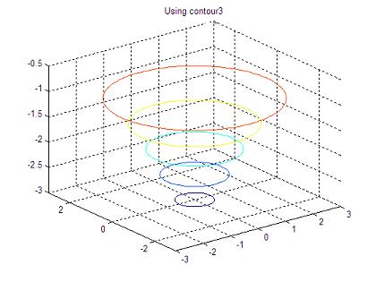
We're plotting exactly the same 3D data (a function depending on two variables) using several instructions, so the visualization is pretty different from each other.

Example:

% cleans the memory workspace

clc; clear; close all;

% defines the range of axes x and y

vx = -3 : 0.1 : 3;

vy = vx;

% generates the powerful grid

[x, y] = meshgrid(vx, vy);

% defines the function to be plotted

z = -10 ./ (3 + x.^2 + y.^2);

% opens figure 1 and plots the function using only contours

figure(1)

contour3(x,y,z)

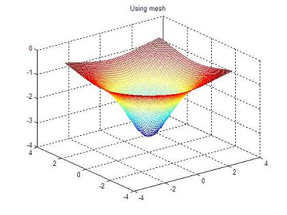
% opens figure 2 and draws the function using a mesh

figure(2)

mesh(x,y,z)

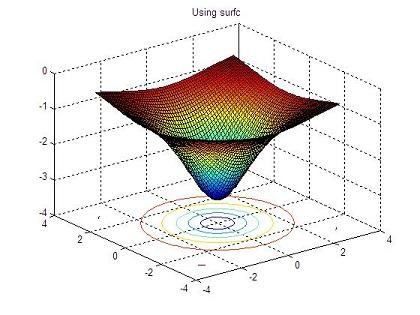
% opens figure 3 and draws the function using surface with contours

figure(3)

surfc(x,y,z)

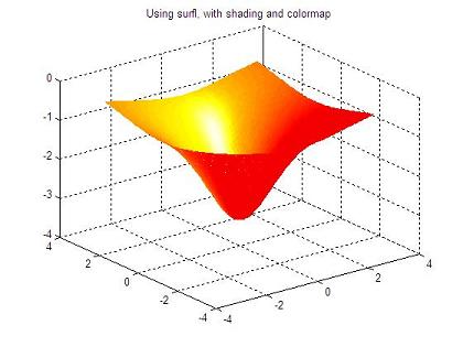
% opens figure 4 and draws the function using a enlightened surface

figure(4)

surfl(x,y,z)

shading interp

colormap hot

The resulting 3D graphics are:

4.3.4 The simple animation in 3d

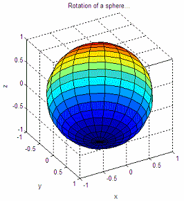
In the first experiment, we are going to work with a sphere and are going to rotate our view angle without changing any size. In the second experiment, we’re going to draw a paraboloid, change its size and rotate. These basic techniques are the foundation of 3D animation with Matlab.

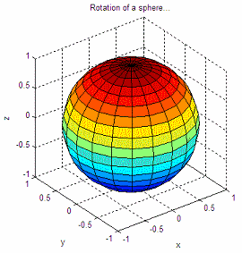
1. Working with a sphere

In this experiment we’re going to draw a sphere and make sure that the axis box keeps its proportions correctly. Then, we’re going to rotate our view angle, i.e., the azimuth and elevation. We are neither moving the sphere itself nor resizing it, we’re just changing our perspective (angle).

Instruction ‘drawnow’ is used to update the current figure. It ‘flushes the event queue’ and forces Matlab to update the screen.

The code that accomplishes this is the following:

clear; clc; close all

% Draw a sphere

sphere

% Make the current axis box square in size

axis('square')

% Define title and labels for reference

title('Rotation of a sphere...')

xlabel('x'); ylabel('y'); zlabel('z')

% Modify azimuth (horizontal rotation) and update drawing

for az = -50 : .2 : 30

view(az, 40)

drawnow

end

% Modify elevation (vertical rotation) and update drawing

for el = 40 : -.2 : -30

view(30, el)

drawnow

end

So we start with this figure:

and after the two soft rotations we end with an image like this:

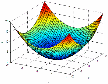
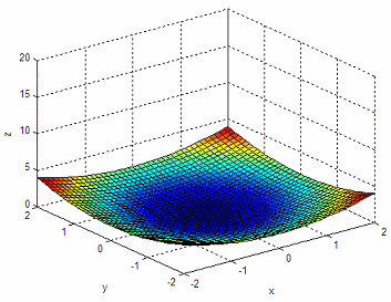
Working with a paraboloid

In our second experiment, we’re going to work with a paraboloid. We first draw it and make sure that the axes have the correct fixed sizes for our purposes. We stretch the figure little-by-little and actually see the change in dimensions. We just update the ‘z’ values within a loop using the function ‘set’ (used to modify the handle graphics properties). Finally, we rotate the azimuth of the figure to achive another view of the box. That’s how we achieve this simple animation in 3D.

The code is the following:

clear; clc; close all

% Define paraboloid

X = -2 : .1 : 2; Y = X;

[x, y] = meshgrid(X, Y);

z = .5 * (x.^2 + y.^2);

% Draw 3D figure, keep track of its handle

h = surf(x,y,z);

% Keep axes constant

axis([-2 2 -2 2 0 20])

% Define title and labels for reference

xlabel('x'); ylabel('y'); zlabel('z')

% Stretch paraboloid and show updates

for i = 1 : .1 : 5;

set(h, 'xdata', x, 'ydata', y, 'zdata', i*z)

drawnow

end

% Modify azimuth (horizontal rotation) and update drawing

for az = -37.5 : .5 : 30

view(az, 30)

drawnow

end

We start with this view:

And we end up with this one: