Антенны, СВЧ / OC / Должиков / Introduction to Smart Antennas_Balanis

DOA ESTIMATION FUNDAMENTALS 73

5.3RECEIVED SIGNAL MODEL

Let us first assume that K uncorrelated sources transmit signals to an N-element antenna array. It is assumed here that the array response for each signal is a function of only one angle parameter (θ ). For our analysis we will employ the well-established narrowband data model. The model inherently assumes that as the signal wavefronts propagate across the array, the envelop of the signal is essentially unchanged [21]. The term narrowband is used under the assumption, satisfied in most of the cases, of a slowing varying signal envelope when either the signals’ or the sensor elements’ bandwidth is small relative to the frequency of operation. This assumption can be also extended to wideband signals, provided the frequency response of the array is approximately flat over the signals’ bandwidth and the propagation time across the array is small compared to the reciprocal bandwidths. Under this model, the received signals can be expressed as a superposition of signals from all the sources and linearly added noise represented by

where x(t) CN is the complex baseband equivalent received signal vector at the antenna array at time t, or

sk (t) is the incoming plane wave from the kth source at time t and arriving from the direction θk , a(θk ) CN is the array response vector to this direction, and n(t) CN represents additive noise. Note that whatever appears in the complex vector n(t) is the noise either “sensed” along with the signals or generated internal to the instrumentation [126]. A single observation x(t) from the array is often referred to as a snapshot. In matrix notation, (5.5) can be written as

where A( ) CN×K is the array response matrix parameterized by the direction of arrival (DOA) (i.e. each column of which represents the array response vector for each signal source), or

is the vector of all the DOAs, or

and s(t) CK represents the vector of the incoming signal in amplitude and phase from each signal source at time t, or

74 INTRODUCTION TO SMART ANTENNAS

Usually, s(t) is referred to as the desired signal portion of x(t). The three most important features of (5.7) are that the matrix A ( ) must be time-invariant over the observation interval, the model is bilinear in A ( ) and s(t), and the noise is additive [21].

The set of array response vectors corresponding to all possible directions of arrival in (5.7), A( ), is also referred to as the array manifold (AM). In simple words, each element ai j (i = 1, 2, . . . , N, j = 1, 2, . . . , K ) of the AM, A ( ), indicates the response of the ith element to a signal incident from the direction of the j th signal. The majority of algorithms developed for the estimate of the DOAs require that the array response matrix A ( ) be completely known for a given parameter vector [127]. This is usually accomplished by direct calibration in the field, or by analytical means using information about the position and response of each individual sensor (such as is done with a uniform linear array, for example).

An unambiguous array manifold A( ) is defined to be one which any collection of K ≤ N distinct vectors from A( ) forms a linearly independent set. For example, an element from the array manifold (an array response vector for a single signal source) of a uniform linear array of identical sensors, as shown in Fig. 5.2, is proportional to

1

e j 2λπ (N−1)d sin θk

where λ is the wavelength of the impinging wavefront and d is the distance between adjacent elements. For a range of angles of arrival θ − π2 , π2 (meaningful for the particular geometry), it is obvious that the AM maintains its unambiguity provided d < λ2 . In the case that θmax < π2 is the maximum bearing deviation from broadside that is expected or imposed by operational considerations, then the wavefield must be sampled at a rate such that d < λ 1 . For more widely spaced sensors, it is possible that there may exist pairs of angles θi and θ j , with θi = θ j ,

such that a(θi ) = a(θ j ). This equality holds when dλ sin θi = n + dλ sin θ j , where n Z, n = 0. In such cases, the array response for a signal arriving from angle θi is indistinguishable from

that arriving from angle θ j .

Uniform sampling of the wavefield implies that all the lags are sampled at least once, and hence, no ambiguous locations should result since the correlation function is completely known [125]. Even though the sampling structure leads to a convenient method of computing a beamformed output by exploiting a structure amenable to FFT processing, it does not need to be uniform [125]. In fact, there may exist cases that it is not required or desirable. Note at this point that the requirement for the interelement spacing in a uniform linear array to be less than

DOA ESTIMATION FUNDAMENTALS 75

half of the wavelength of the highest frequency in the receiver band can be interpreted as the spatial analog to the well-known Nyquist sampling criterion which allows the reconstruction of a continuous-time wavefront occupying a bandwidth B from its discrete-time samples if these are taken with sampling frequency of not less than 2B. If A ( ) is unambiguous and N ≥ K , then A ( ) will be of full-rank K . In a similar manner, for an array manifold with resolved ambiguity, knowing the mode vector a(θi ) is tantamount to knowing the angle θi [126].

Furthermore, for a set of data observations L > K , we can form the matrices

5.4THE SUBSPACE-BASED DATA MODEL

Ignoring the noise effects in (5.13), each observation of the received signal, A ( ) S, is constrained to lie in the K -dimensional subspace CN defined by the K columns of A ( ).

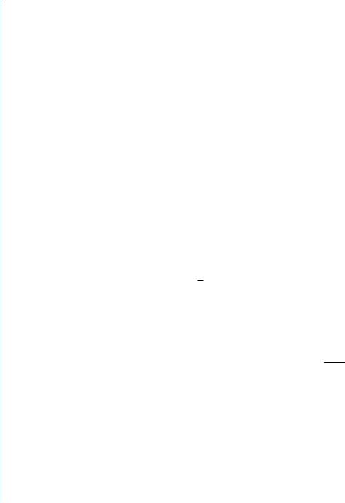
Fig. 5.3 illustrates this idea for the special case of two sources (K = 2) and four snapshots (L = 4). Each of the two sources has associated with it a response vector a (θk ) from the array manifold, and the four snapshots x(t1), . . . , x(t4) lie in the two-dimensional subspace spanned by these vectors. The specific positions of these vectors depend on the signal waveforms at each time instant. Note that the array manifold intersects the signal subspace at only two points, each corresponding to a response of one of the signals [21].

Even though L > K , it is possible, however, for the signal subspace to have dimension smaller than K . This occurs if the matrix of signal samples S has a rank less than K . This situation may arise, for example, if one of the signals is a linear combination of the others. Such signals are referred to as coherent or fully-correlated signals, and occur most frequently in the sensor array problem in a multipath propagation scenario. Multipath results when a given signal is received at the array from several different directions or paths due to reflections from various objects in the wireless channel. It may also be possible that the available snapshots are fewer than the emitting sources, in which case the signal subspace cannot exceed the number of observations [21]. In either case, the dimension of the signal subspace is less than the number of present sources. However, this does not imply that estimates of the number of sources are impossible. For instance, it can be shown [126] that for one-parameter vectors, the angle of arrival in our case (or any other one parameter per source), the signal parameters are still identifiable if A ( ) is unambiguous and N > 2K − K , where K = rank [A ( ) S].

76 INTRODUCTION TO SMART ANTENNAS

Signal

Subspace

x(t1)

x(t2)

x(t4)

x(t3)

Array

Manifold

FIGURE 5.3: A geometric view of the DOA estimation problem [21].

The identifiability condition, geometrically obvious, is that the signal subspace be spanned by a unique set of K vectors from the array manifold.

In the event that the measurements made are more than the present signals (i.e., the number of sources K is less than the number of elements N), the data model in (5.7) admits an appealing geometric interpretation and provides insight into the sensor array processing problem [21]. The measurements taken form the vectors of complex values with dimension in space equal to the number of elements in the array (N). In the absence of noise, the expression which gives x(t) in (5.7), A ( ) s(t), is confined to a space dimension K (at most a K -dimensional subspace of CN ), referred to as the signal subspace and it spans either the entire or some fraction of the column space of A ( ). If any of the impinging signals are perfectly correlated, i.e., one signal is simply complex scalar multiple of another, the span of the signal subspace K will be less than K . Consequently, if there is sufficient excitation, in other words no signals are perfectly correlated, the signal subspace is K -dimensional. Considering noise, since it is typically assumed to possess energy in all dimensions of the observation space, (5.7) is often referred to as a low-rank signal in full-rank noise data model.

This entire geometric picture leads to the accurate parameter estimation problem by handling it as subspace intersection. Because of the many applications for which the subspacebased data method is appropriate, numerous subspace-based techniques have been developed to exploit it [21].

DOA ESTIMATION FUNDAMENTALS 77

5.5SIGNAL AUTOCOVARIANCE MATRICES

Before we discuss the algorithms for DOA estimation, we first need to define two commonly used terms: the received signal autocovariance matrix Rxx and the desired signal autocovariance matrix Rs s given by

where H denotes Hermitian (or complex-conjugate transpose) matrix operation and E{·} is the expectation operation on the argument. In reality, the expected value cannot be obtained exactly since an infinite time interval is necessary and estimates, as the average over a finite, sufficiently enough, number of data “snapshots” must be used in practical implementations as

ˆ

The same approximation holds for Rs s . With the typical assumption that the incident signals are noncoherent, the source covariance matrix Rs s is positive definite [128]. In addition, the noise is typically assumed to be a complex stationary Gaussian random process. The motivation for this assumption is that if there are many sources of noise, the sum will be Gaussian distributed according to the central limit theorem [129]. Also, further analysis of direction finding performance is greatly simplified by assuming white Gaussian noise.

If, additionally, it is assumed to be uncorrelated both with the signals, and for successive signal samples, (5.14) can be written as

where σn2 is the noise variance and is normalized so that det ( ) = 1. The simplifying assumption of spatial whiteness (i.e., = I, where I is the identity matrix) is often made.

The assumptions of a known array response and known noise covariance are never practically valid. Due to changes in the weather, reflective and absorptive bodies in the nearby surrounding environment, and antenna location, the response of the array may be substantially different than it was last calibrated [130]. Furthermore, the calibration measurements themselves are subject to gain and phase errors. For the case of analytically calibrated arrays of identical elements, including orientation, errors may occur because the elements are not really identical and their locations are not precisely known. Depending on the degree to which the actual antenna response differs from its nominal value, the performance of a particular algorithm may significantly be degraded [130].

78 INTRODUCTION TO SMART ANTENNAS

Since the surrounding environment of the array may be time-varying, the requirement of known noise statistics is also difficult to satisfy in practice. In addition, effects of unmodeled “noise” phenomena such as distributed sources, reverberation, noise due to the antenna platform, and undesirable channel crosstalk are often unable to be accounted for. Measurement of the noise statistics is usually a complicated task due to the fact that signals-of-interest are often observed along with the noise and interference. When signal subspace methods are applied for DOA estimation, it is often assumed that the noise field is isotropic, independent from channel to channel and equal at each one [130], which is not the case in reality. For high signal-to-noise (SNR) ratio, deviations of the noise from these assumptions are not critical since they contribute little to the statistics of the received by the array signal. However, at low SNR values, the degradation in the algorithms’ performance may be severe.

5.6CONVENTIONAL DOA ESTIMATION METHODS

Two methods are usually classified as conventional methods: the Conventional Beamforming Method and Capon’s minimum Variance Method [13].

5.6.1Conventional Beamforming Method

The conventional beamforming method (CBF) is also referred to as the delay-and-sum method or Bartlett method. The idea is to scan across the angular region of interest (usually in discrete steps), and whichever direction produces the largest output power is the estimate of the desired signal’s direction. More specifically, as the look direction θ is varied incrementally across the space of access, the array response vector a(θ ) is calculated and the output power of the beamformer is measured by

This quantity is also referred to as the spatial spectrum and the estimate of the true DOA is the angle θ that corresponds to the peak value of the output power spectrum.

The method is also referred to as Fourier method since it is a natural extension of the classical Fourier based spectral analysis with different window functions [131, 132]. In fact, if a ULA of isotropic elements is used, the spatial spectrum in (5.18) is a spatial analog of the classical periodogram in time-series analysis. Note that other types of arrays correspond to nonuniform sampling schemes in time-series analysis. As with the periodogram, the spatial spectrum has a resolution threshold. That is, an array with only a few elements is not able to form neither narrow nor sharp peaks and hence, its ability to resolve closely spaced signals

80 INTRODUCTION TO SMART ANTENNAS

is equal to the number of array elements N. The received signal space can be separated into two parts: the signal subspace and the noise subspace. The signal subspace is the subspace spanned by the columns of A ( ) [21], and the subspace orthogonal to the signal subspace is known as the noise subspace. The subspace algorithms exploit this orthogonality to estimate the signals’ DOAs.

5.7.1The MUSIC Algorithm

Within the class of the so-called signal-subspace algorithms, MUSIC (MUltiple SIgnal Classification)[123, 135] has been the most widely examined. In a detailed performance evaluation based on hundreds of simulations, MIT’s Lincoln Laboratories concluded that, among the high-resolution algorithms then available, MUSIC was the most promising and a leading candidate for further study and actual hardware implementation [136].

The popularity of the MUSIC algorithm is in large part due to its generality. For example, it is applicable to arrays of arbitrary but known configuration and response, and can be used to estimate multiple parameters per source (e.g., azimuth, elevation, range, polarization, etc.). However, this generality is accompanied with the expense that the array response must be known for all possible combinations of source parameters; i.e., the response must be either measured (calibrated) and stored, or one must be able to characterize it analytically (e.g., as in the case of root-MUSIC [123, 137]). In addition, MUSIC requires a priori knowledge of the second-order spatial statistics of the background noise and interference field. These assumptions are never satisfied in reality as explained earlier.

The MUSIC algorithm was developed by Schmidt [123, 126] by noting that the desired signal array response is orthogonal to the noise subspace. The signal and noise subspaces are first identified using eigendecomposition of the received signal covariance matrix. Following, the MUSIC spatial spectrum is computed, from which the DOAs are estimated. Inside the algorithm, we first define the general array manifold to be the set

for some region of interest in the DOA space. The array manifold is assumed unambiguous and known for all the values of angle θ , either analytically or through some calibration procedure. The objective is to apply appropriate methods to the received signals so as to extract the region θ out of the range of .

If noise was absent in (5.7), the observations x(t) would be confined entirely to the K -dimensional subspace of CK defined by the span of A ( ). Determining the DOAs for the no-noise case is simply a matter of finding the K unique elements of A that intersect this subspace [130]. A different approach is necessary in the presence of noise since the observations become “full-rank”. The approach of MUSIC, and other subspace-based methods, is to first

DOA ESTIMATION FUNDAMENTALS 81

estimate the dominant subspace of the observations, and then find the elements of A that are in some sense closest to this subspace.

The subspace estimation step is typically achieved by eigendecomposition of the autocovariance matrix of the received data Rxx . For MUSIC to be applicable, the emitter covariance Rs s is required to be full-rank, i.e., that K = K . Using the model in (5.17) and assuming spatial whiteness2, i.e., E n(t)nH (t) = σn2I, the eigendecomposition of Rxx will give the eigenvalues λn such that λ1 > λ2 > . . . > λK > λK +1 = λK +2 = . . . = λN = σn2 and the corresponding eigenvectors en CN , n = 1, 2, . . . , N, of Rxx . Furthermore, it is easily shown that Rxx can be written in the following form [138]:

diag {λ1, λ2, . . . , λN }, s = diag {λ1, λ2, . . . , λK }, n = diag {λK +1, λK +2, . . . , λN }, and

(i.e., EEH = EH E = I). The span of the K vectors Es defines the signal subspace, and the orthogonal complement spanned by En defines the noise subspace. For a detailed analysis of the eigenstructure properties of the signal autocovariance matrices Rxx and Rs s the reader is referred to [126]. Once the subspaces are determined, the DOAs of the desired signals can be estimated by calculating the MUSIC spatial spectrum over the region of interest [21]:

Note that the a(θ )s are the array response vectors calculated for all angles θ within the range of interest. Because the desired array response vectors A ( ) are orthogonal to the noise subspace, the peaks in the MUSIC spatial spectrum represent the DOA estimates for the desired signals. Due to imperfections in deriving Rxx , the noise subspace eigenvalues will not be exactly equal to σn2. They do, however, form a group around the value σn2 and can be distinguished from the signal subspace eigenvalues. The separation becomes more pronounced as the number of samples used in the estimation of Rxx increases (ideally reaches infinity).

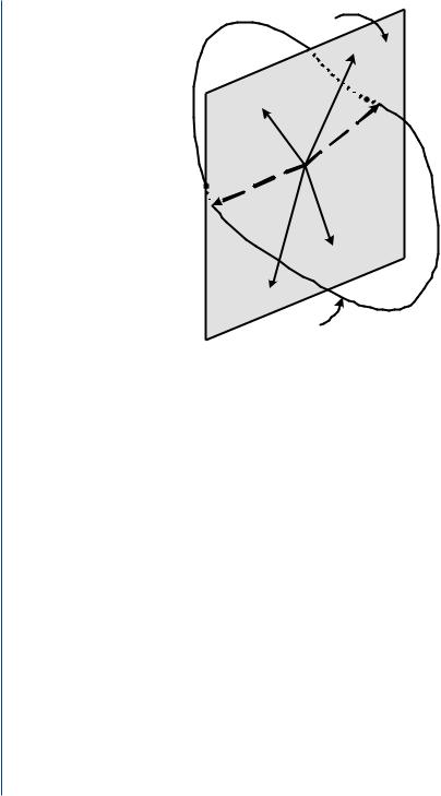
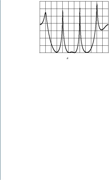
To demonstrate the efficiency of the algorithm, we choose as an example a ULA with N = 8 and d = λ/2. We assume four equal-power uncorrelated sources (K = 4) located in the far-field of the array, with θ1 = +60◦, θ2 = +15◦, θ3 = −30◦, and θ4 = −75◦. Moreover,

2The assumption of spatially white noise is not necessary; the extension to an arbitrary noise autocovariance σn2 = is straightforward, provided that is known.

82 INTRODUCTION TO SMART ANTENNAS

FIGURE 5.4: Spatial spectrum of the MUSIC algorithm.

uncorrelated spatially white Gaussian noise with zero mean and unit variance (σn2 = 1) is assumed. A total of 500 observations are taken (L = 500). Fig. 5.4 displays the obtained MUSIC spatial spectrum. The performance of the algorithm is shown to be excellent, since the peaks in the spatial spectrum are located at angles being exactly the DOAs.

A final remark for the algorithm’s performance is that MUSIC yields asymptotically unbiased parameter estimates, even for multiple incident wavefronts, because both Rs s and En are asymptotically perfectly measured [139].

5.7.2The ESPRIT Algorithm

Although the performance advantages of MUSIC are substantial, they are achieved at a considerable cost in computation (searching over parameter space) and storage (of array calibration data). Moreover, even for the one-dimensional MUSIC estimation (DOA in the particular case), there exist several drawbacks although being conceptually easy. Primarily, problems in the finite measurement case arise from the fact that since K signals are known to be present, the search for their DOAs, (θ1, θ2, . . . , θK ), should be sought simultaneously by maximizing an appropriate functional rather than obtaining estimates one at a time as is done in the search for spectral peaks over PMU S I C (θ ). However, multidimensional searches are accompanied with an intense expense compared to one-dimensional searches. The reduction in computational load achieved with an one-dimensional search for K parameters comes with the trade-off of the method being finite-sample-biased in a multisource environment [122]. Furthermore, in either low SNR scenarios or closely spaced sources (i.e., multiple peaks observed in the measurements) MUSIC’s performance reduces dramatically. Nevertheless, despite its drawbacks, it should be